Download
1 / 28
280 likes | 438 Vues
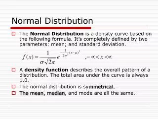
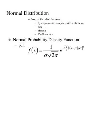
Normal Distribution. Sampling and Probability. Properties of a Normal Distribution. Mean = median = mode There are the same number of scores below and above the mean. 50% of the scores are on either side of the mean. The area under the normal curve totals 100%.

E N D
Normal Distribution Sampling and Probability
Properties of a Normal Distribution • Mean = median = mode • There are the same number of scores below and above the mean. • 50% of the scores are on either side of the mean. • The area under the normal curve totals 100%..
Not all distributions are bell-shaped curves • Some distributions lean to the right • Some distributions lean to the left • Some distributions are tall or peaked • Some distributions are flat on top
Things to remember about skewed distributions • Most distributions are not bell-shaped. • Distributions can be skewed to the right or the left. • The direction of the skew pertains to the direction of the tail (smaller end of the distribution). • Tails on the right are positively skewed. • Tails on the left are negatively skewed.
Other things to know about skewness • Skewness is a measure of how evenly scores in a distribution are distributed around the mean. • The bigger the skew the larger is the degree to which most scores lie on one side of the mean versus the other side. • Skew scores produced in SPSS are either negative or positive, indicating the direction of the skew.
Knowing whether a distribution is skewed: • Tells you if you have a normal distribution. (If the skew is close to zero, you may have a normal distribution) • Tells you whether you should use mean or median as a measure of central tendency. (The greater the skew, the more likely that the median is the better measure of central tendency) • Tells you whether you can use inferential statistics.
Another measure of the shape of the distribution is kurtosis. This measure tells you: • Whether the standard deviation (degree to which scores vary from the mean) are large or small) • Curves that are very narrow have small standard deviations. • Curves that are very wide have large standard deviations. • A kurtosis measure that is near zero (less than 1) may indicate a normal distribution.
Other Important Characteristics of a Normal Distribution • The shape of the curve changes depending on the mean and standard deviation of the distribution. • The area under the curve is 100% • A mathematical theory, the Central Limit Theorem, allows us to determine what scores in the distribution are between 1, 2, and 3 standard deviations from the mean.
Central Limit Theorem: • 68.25% of the scores are within one standard deviation of the mean. • 94.44% of the scores are within two standard deviations of the mean. • 99.74%(or most of the scores) are within 3 standard deviations of the mean.
Central Limit Theorem also means that: • 34.13% of the scores are within one standard deviation above or below the mean. • 47.12% of the scores are within two standard deviations above or below the mean. • 49.87% of the scores are within three standard deviations above or below the mean.
This theory allows us to: • Determine the percentage of scores that fall within any two scores in a normal distribution. • Determine what scores fall within one, two, and three standard deviations from the mean. • Determine how a score is related to other scores in the distribution (What percentage of scores are above or below this number). • Compare scores in different normal distributions that have different means and standard deviations. • Estimate the probability with which a number occurs.
Determining what scores fall within 1, 2, and 3 SD from the Mean
To do some of these things we need to convert a specific raw score to a z score. A z score is: • A measure of where the raw score falls in a normal curve. • It allows us to determine what percentage of scores are above or below the raw score.
The formal for a z score is: (Raw score – Mean) Standard Deviation If the raw score is larger than the mean, the z score will be positive. If the raw score is smaller than the mean, the z score will be negative. This means that when we try to compare the raw score to the distribution, a positive score will be above the mean and a negative score will be below the mean!
For example, (Assessment of Client Economic Hardship) Raw Score = 23 Mean = 25 SD = 1.5 23-25- 2 = - 1.33 1.5 1.5 Percent of Area Under Curve = 40.82%
But where does this client fall in the distribution compared to other clients. What percent received higher scores?What percent received lower scores?
To convert z scores to percentages; • Use the chart (Table 8.1) on p. 132 of your textbook (Z charts can be found in any statistics book). • Area under curve for a z score of -1.33 is 40.82
To find out how many clients had lower or higher economic hardship scores: Lower Scores – Area of curve below the mean = 50% 50% – 40.82% = 9.18% Consequently 9.18% had lower scores. Higher scores = 40.82% + 50% (above the mean) = 90.82% had higher scores.
Positive Z score example: Raw Score = 15 Mean = 12 Standard Deviation = 5 = 15 – 12 = 3 = .60 = 22.57 5 5 50 – 22.57 = 27.43% had higher scores on the economic hardship scale 50 + 22.57 = 72.57 had lower scores on the scale
How do scores from different distributions compare: Distribution 1 Raw Score = 10 Mean = 5 SD = 2 = 10 – 5 = 5 = 2.5 = 49.38 = .62% above 2 2 99.38% below Distribution 2 Raw Score= 9 Mean = 4 SD = 2.2 = 9 - 4 = 5 = 2.27 = 48.84 = 1.16% above 2.2 2.2 98.84% below