Download
1 / 21
220 likes | 349 Vues
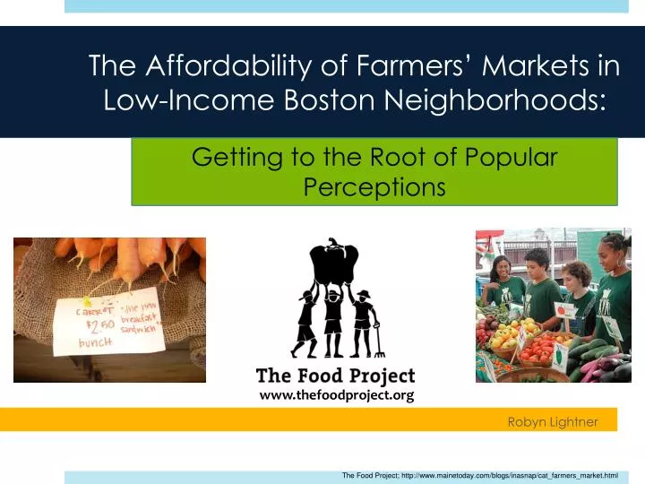
Getting to the Root of Popular Perceptions . The Affordability of Farmers’ Markets in Low-Income Boston Neighborhoods:. Robyn Lightner. www.thefoodproject.org. The Food Project; http://www.mainetoday.com/blogs/inasnap/cat_farmers_market.html. Introduction.

E N D
Getting to the Root of Popular Perceptions The Affordability of Farmers’ Markets in Low-Income Boston Neighborhoods: Robyn Lightner www.thefoodproject.org The Food Project; http://www.mainetoday.com/blogs/inasnap/cat_farmers_market.html
Introduction • By 2010, 21 farmers’ markets throughout the Boston metropolitan area participated in the BBB program and the usage of SNAP ($41,402.28) along with BBB matches ($36,409.46) combined for a total of $77,811.74 in sales- a 387% increase over the previous summer. • Representing 28.5% of total Boston sales, the ten FM located in Dorchester and Roxbury reported a total of $21,699.58 in combined SNAP/BBB sales (The Food Project, preliminary report, 2011). • BUT, there remains a widespread perception that farmers’ market produce is more expensive than conventional supermarket produce. This uninformed perception is a barrier to the attendance of price-sensitive shoppers at farmers’ markets.
Relative Cost of Direct Retail • Problems with previous research: did not devise plan to handle multi-leveled inconsistency of produce, combined produce into market basket, short time frame ignored effects of seasonality and volume. • Demonstrated need for a replicable methodology for comparing produce prices at conventional grocery outlets with those at direct retail outlets • Must be neighborhood-specific, include strategies that account for hard to measure effects of seasonality and quality Pie Chart Comparing Prices at Seattle Farmers Markets with Prices at QFC (SM) Pirog and McCann, 2009; Kaemingk, 2010.
Observational Study Objective • Clarify perception that farmers market produce is more expensive than conventional market produce in order to accurately educate communities about the local affordability of healthy food & inform the efforts of community groups, policy advocates, farmers, etc. • Learn how the price of produce differs between farmers’ markets and supermarkets in Dorchester and Roxbury • Focus on specifics of a well-defined geographic/demographic area • Assess relative quality between locations
Methods: Variable Selection Neighborhoods • North Dorchester, South Dorchester, Roxbury • Similar socio-economic statistics, outlet density, momentum Retail Outlets • All 10 FM and 7 SM in 8 mile area • FM implemented for variety of reasons • All outlets accept SNAP/EBT, WIC; all FM accept FMNP and BBB Time Periods • Eight 14-day periods between July 5 and October 24, 2010 Vendor Research • Organic certification, time between point of harvest and sale, pricing strategies Dorchester Roxbury = Farmers Market = Supermarket
Methods: Variable Selection Produce Types • Carrots: unpeeled, with green tops and w/o green tops • Cucumbers: unwrapped, not English • Onions: yellow, large, loose (not bagged) • Tomatoes (field): about fist size, not hot house/ greenhouse, not heirloom, no vine • Zucchini: green summer squash • White Potatoes: loose • Scallions: green onions (not red bulb) • Lettuce: green leaf, not romaine/Bibb/iceberg variety, not bagged/washed/trimmed • Bell Peppers (green): loose • Green Beans: loose Bowdoin Street Health Center; Robyn Lightner
Methods: Data Collection • All observations were taken within the same 14-day period • Recorded price/lb. data for the smallest, most conventional (i.e. non-organic) unit sold • If non-pound unit, recorded unit price and took RS of unit weight to be converted into price/lb. • Ranked overall visual quality of the produce item using a scale of 1 to 3 • All data collectors went through training workshop in order to ensure consistency • Many problem-specific strategies
Description of Data • Only 45% of possible observations at FM were actually realized and included in the final data set, compared with 88% of possible observations at SM. • Both location types have fairly equal representation in the final data set • An unrealized data point most commonly resulted from the case that a certain produce item was not available at the time or day of data collection, but may have also been the consequence of misreported data, a sold out item, or market cancellation due to weather, among others. • The variance of mean price per pound at FM (0.904) was significantly lower (p = .026) than the variance for the same value at SM (0.985), meaning that overall variation in mean price per pound was greater at SM. • Mean quality at FM (2.74) was significantly higher (p < 0.00) than at SM (2.46) by .27, or about 11%. • The standard deviation of quality rating was also lower at FM (0.47) than at SM (0.62), indicating that SM reported greater variation in quality.
Data Analysis Multivariate Regression Model Y = lnPRICE = 0 + 1 LOC + 2 TIME1 + … + 8 TIME7 + 9 PROD1 + … + 17 PROD9 + 18 QUAL1 + 19 QUAL2 + E • “How does the mean price per pound (PRICE) change with variation in location type (LOCATION), while produce type (PRODUCE), time period (TIME), and quality rating (QUALITY) are held constant?” • Results verified using log transformation to enhance normality of distribution • Statistical analyses were performed using STATA, version 9.0 (StataCorp, College Station, TX, 2008).
Regression Model Regression Summary of lnPRICE on Successive Fixed Effects • A regression of the dependent variable lnPRICE on LOCATION controlling for PRODUCE, TIME, and QUALITY yields anestimated coefficient of .029 and a p-value of 0.043. These results suggest that when produce type, time period, and quality are held constant, the price per pound is 2.9% greater at farmers’ markets. The very low p-value of .043 asserts the statistical significance of this result.
Time Period Time Period Time Period Time Period Time Period Time Period Regression by Time & Produce Type
Other Discount Opportunities • Bulk discounts • i.e. Shaw’s loose onions were sold for $1.79/lb. compared with a 2 lb. package of onions for $0.92/lb (about a 50% discount), and Tropical Foods sold loose potatoes for $0.79/lb. compared with a 5 lb. bag for $0.34/lb (nearly a 60% discount). • Value card discounts • i.e. “Stop and Shop Card” offered zucchini for $0.50/lb. (regular price = $1.49) or green beans for $0.20/lb. (regular price = $1.69). • Bounty Bucks • Up to $10.00 in “free” produce for SNAP users
More on Quality • Organic or IPM Growing Methods • 2 vendors certified (Langwater and Serving Ourselves), all others practice mostly organic growing methods • Freshness • All produce was grown within 2 hours driving time of Boston • Likely sold within 24-48 hours of harvest Examples of Comments on Quality
How Much Really is 3%? • The Economic Research Service of the USDA recently announced that an adult on a 2,000-calorie diet could satisfy recommendations for fruit and vegetable consumption in the 2010 Dietary Guidelines for Americans at an average of $2 to $2.50 per day (Stewart et al., 2008). • Using a mean of $2.25, an increase by 3% would increase daily cost of consuming the recommended F & V amount by about 7-cents to $2.32. • Over the course of the 16-week/112 day summer market season used in this study, purchasing the recommended daily amount of produce would increase from $252.00 to $259.84- just under $8.00 over 4 months. • This added expense could be more than compensated for in just one day using Bounty Bucks!
How can this information be used to educate consumers about the affordability of neighborhood farmers’ markets? • Focus on the seasonal height of specific produce types and use time-sensitive publicity to encourage purchasing when price is lowest. For example, highlight bell peppers and cucumbers as “Top Pickings” or “Highest Seeds” during the last two weeks of September (time period 6), and do the same for scallions and lettuce during the first two weeks in October (time period 7). • Create a citywide graphic that shows a visual of how much produce $20 could get a SNAP user at farmers’ markets and how that produce translates into a few days worth of vegetable servings. • Create a side-by-side visual comparison of the amount of produce a shopper could buy using $10 worth of SNAP at a supermarket, then show that same amount doubled for farmers’ markets to demonstrate the double voucher benefits available through Boston Bounty Bucks.
Special Thanks • Cammy Watts, The Food Project • Cathy Wirth, Bowdoin Street Community Health Center • Professors Kate Sims, Jan Dizard, and Amy Wagaman, Amherst College • Phuong Luong and Cara Brumfeld, The Food Project • Nebi Stephens, Cynthia Loesch, Tim Deihl, Dave Dumaresque, The B.O.L.D. Teens of Codman Square http://www.boldteens.org/media.html