Download

1 / 20
200 likes | 363 Vues
Comparing 2 population parameters. Chapter 13. Introduction: Two Sample problems.

E N D
Comparing 2 population parameters Chapter 13
Introduction: Two Sample problems • Ex: How do small businesses that fail differ from those that succeed? Business school researchers compare the asset to liability ratios of 2 samples of firms started in 2000: one sample of failed businesses and one of firms still going strong. • This observational study compares two random sample, one from each of two different populations. • Comparing two populations or two treatments is one of the most common situations in statistical practice.
13.1 We can examine two-sample data graphically by comparing dotplots or stemplots (smaller samples) or histograms or boxplots (larger samples). This chapter details Note! The difference between independent samples (this chapter) and matched pairs or paired samples (past chapters)
Conditions for comparing 2 means *Note: If each population is normally distributed, then μ1 – μ2 will be too
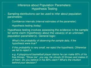
Symbols There are four unknown parameters (the two means and the two SD’s). We want to compare the two population means, either by giving a confidence interval for their difference (μ1 – μ2) or by testing the hypothesis of no difference, H0: μ1 = μ2
Two Sample Z Statistic • If we know the population standard deviations for both groups (unlikely) we use a 2 sample Z test. By hand (formula below, same as before) or on calc (2-SampZTest)
Two Sample T Test • Degrees of freedom for T*: Complicated to calculate, so 2 options • 1. Calc does it automatically! (decimals possible • 2. Compare the df of each sample (n1 – 1) and (n2 – 2). Use the smaller of the 2 groups. This is very conservative.
Robustness • The 2 sample t procedures are more robust than the one-sample t methods • When planning a two sample study, choose equal sample sizes if you can. When the shapes of the 2 populations are similar and the two samples are equal sizes, p – values are quite accurate. • Two sample t procedures are most robust against non-Normality and the conservative P-values (using option 2 for df) are most accurate.
Example • Does increasing the amount of calcium in our diet reduce blood pressure? • Double Blind, Randomized comparative experiment with 21 healthy men. Group 1, chosen randomly, 10 men receiving a calcium supplement for 12 weeks. Group 2, 11 men, received an identical placebo. • Response variable: The decrease in systolic blood pressure for the subject after 12 weeks in MM of Mercury (so a negative # indicates an increase Group 1: 7, -4, 18, 17, -3, -5, 1, 10, 11, -1 Group 2: -1, 12, -1, -3, 3, -5, 5, 2, -11, -1, -3
1: Hypothesis • H0: μ1 =μ2 or H0: μ1 -μ2 = 0 HA: μ1 ≠ μ2 HA: μ1 -μ2 ≠ 0 2: Conditions • SRS: Assume random selection of 21 subjects from population of all men, and random assignment of subjects to treatments confirmed in • Normality: Small samples, check plots of each (no serious non-normality or huge outliers)
Independence: “Because of the randomization, we are willing to regard the calcium and placebo groups as two independent samples. We are not sampling without replacement from a population of interest in this case. • 3. Calculations: We use the T test b/c we don’t know population sigma P value: There are 9 DF (the smaller of the 2 groups) which is approximately .07
4: Interpretation The experiment provides some evidence that calcium reduces blood pressure, but the evidence falls short of the traditional 5% and 1% levels. We would fail to reject the null at either of these significance levels. 90% Confidence interval: (t* is 1.833) (-.753, 11.299). We are 90% confident that the true mean advantage of calcium over a placebo lies in this interval. Since 0 is in the interval, we cannot reject the null. *Remember, these are small samples! Bigger samples (and bigger df) give smaller t* values making them easier to ‘beat’ and attain significance!
Calculator • Enter Group 1 data into L1 and Group 2 into L2 • Go to Stat/Tests choose 2-SampTTest • Specify “data” Pooled- NO • CI: Choose 2-SampTInt then data, etc • “Pooled”: DON’T POOL!!!
13.2 Comparing 2 proportions • Ex: Does prayer help with in vitro fertilization? Through random assignment, 88 women undergoing in vitro were prayed for by intercessors and 81 were not. 44 of the 88 women (50%) in the treatment group got pregnant compared to 21 out of the 81 (26%) in the control group. This difference seems large, but is it statistically significant?
Symbols We compare the populations by doing inference about the difference ρ1 - ρ2
Calculator • Significance test: 2-PropZtest • CI: 2-PropZInt
Let’s do In Vitro Example • 1: Hypothesis • H0:ρ1= ρ2 or H0: ρ1 -ρ2 = 0 HA: ρ1≠ ρ2 HA: ρ -ρ2 ≠ 0 • 2: Conditions • SRS? Normality? Independence? • 3: Calculations (on calc) • 4: Interpretation • “This study shows that intercessory prayer may cause an increase in pregnancy. However, it is unclear if the women knew that they were in a treatment group. If they found out that other people were praying for them, then their behaviors may have changed.
Continued • CI on calc + interpretation • Explain Type I and Type II error in this setting. Which is more serious?