Download
1 / 26
270 likes | 453 Vues
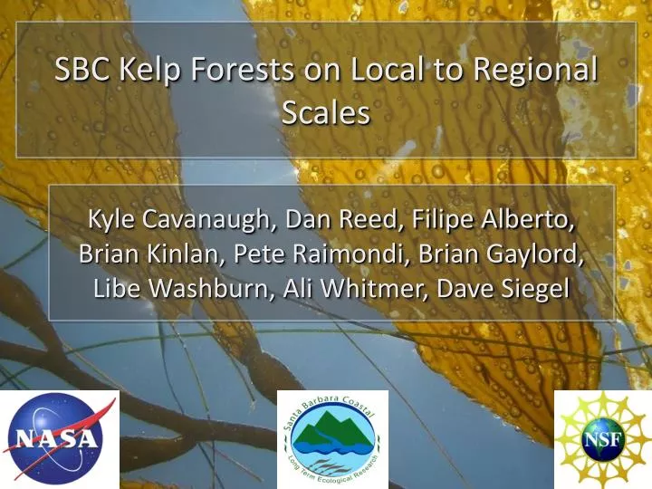
SBC Kelp Forests on Local to Regional Scales. Kyle Cavanaugh, Dan Reed, Filipe Alberto, Brian Kinlan, Pete Raimondi, Brian Gaylord, Libe Washburn, Ali Whitmer, Dave Siegel. Giant Kelp Characteristics. Plant life spans: 2 to 3 years Frond life spans: about 4 months

E N D
SBC Kelp Forests on Local to Regional Scales Kyle Cavanaugh, Dan Reed, Filipe Alberto, Brian Kinlan, Pete Raimondi, Brian Gaylord, Libe Washburn, Ali Whitmer, Dave Siegel
Giant Kelp Characteristics Plant life spans: 2 to 3 years Frond life spans: about 4 months Frond growth can be 0.5 m/day Leads to highly dynamic population dynamics
What Controls Giant Kelp Biomass? NUTRIENTS & TEMPERATURE: ocean processes affecting growth rates & spore production PHYSICAL DISTURBANCE: waves & currents removing fronds and/or holdfasts, changes in benthic type (rock to sand) GRAZING: urchins on plants, filter feeders on spores, etc. SENESCENCE: natural loss of fronds due to age HUMANS: harvesting, pollution, etc.
Site based measurements of kelp forest structure and dynamics are key component of SBC LTER long term data Data on > 150 species collected in permanent plots at 20 sites in the Santa Barbara Channel.
Surveys provide important information about demographic processes Surveys do NOT provide a regional view of kelp forest dynamics Need to combine field & satellite observations to understand local to regional scale dynamics Sampling Forests from Fixed Surveys SPOT 5 analysis by Cavanaugh et al. MEPS [2010]
LANDSAT 5 Imagery Santa Barbara AQUE MOHK • 30 m resolution multispectral imagery • Available from 1984-present with a 16 day repeat cycle • Cloud free image every ~6 weeks • Imagery are now free Cavanaugh et al. MEPS, in review.
LANDSAT 5 Spectral Analysis Atmospheric correction (fixed target method) Model each pixel as a linear combination of water & kelp endmembers (following Dennison & Roberts, 2003) Single kelp & multiple water endmembers (used to account for variable sediment, glint, phytoplankton, etc.)
Examples of Spectral Unmixing clear/quiescent glint plumes 10/02/2004 07/04/2006 02/23/2005
Biomass from LANDSAT Transect Biomass (kg/m2) r2 = 0.62 p < 0.001 LANDSAT Kelp Fraction Strong relationship between kelp fraction and diver measured canopy biomass
Regionl Scale Giant Kelp Dynamics over the SB region x 108 2.0 1.5 El Nino El Nino Biomass (kg) 1.0 1988 1984 1986 1990 2004 2006 1992 1994 1996 1998 2000 2002 2008 2010 0.5 0 Regional mean: ~40,000 metric tons of kelp canopy Low in winter, high in summer/fall Annual cycle superimposed on a 11-13 year cycle
Physical Data Pt. Arguello buoy Santa Barbara Harvest buoy SST is a good proxy for nutrients Significant wave height from Harvest buoy (1987-2009) Sea Surface Temperature (SST) from Pt. Arguello buoy (1984-2009)
Seasonal Forcing • Wave induced mortality is direct and immediate • Effect of SST/nutrients is delayed and complicated by other factors Spring/Summer Recovery Winter Loss 19 100 r2 = 0.30 p = 0.01 80 18 60 Percent Loss log(growth) 17 40 r2 = 0.50 p < 0.01 20 16 7 8 16 15 3 5 6 4 12 14 13 Max Wave Height (m) Mean SST (°C)
Interannual Forcing NPGO PDO ENSO -5 -4 -3 -2 -1 0 1 2 3 4 5 -5 -4 -3 -2 -1 0 1 2 3 4 5 -5 -4 -3 -2 -1 0 1 2 3 4 5 Lag (years) Max Wave Height Mean SST Correlation w/ kelp -5 -4 -3 -2 -1 0 1 2 3 4 5 -5 -4 -3 -2 -1 0 1 2 3 4 5
Kelp population controls wave height NPGO + wave height - - + biomass nutrients nutrients + + - biomass + recruitment -48 -36 -24 -1 0 time (months)
Subregional Variability mean biomass (kg/m2) Mean kelp cover biomass (kg/m2) Pt. Conception Santa Barbara • Bin kelp into 1 km coastline segments • K-means clustering
Cluster Analysis Long Period Swell Which 1 km time series are more similar to each other? (assumes 4 clusters) winter Hs winter swells summer summer swells Correlation with physical variables periods > 12 sec
Kelp Forests as a Metapopulation Metapopulation: collection of small, discrete populations (patches) connected via dispersal Patches undergo transitions as they are colonized, grow/shrink & become extinct Key metrics include isolation, persistence, connectivity, etc. Appropriate for kelp due to patchy nature and responses to disturbance
50 40 30 Relative frequency (%) PDO cool Pacific Decadal Oscillation warm 20 10 0 0 1 2 3 4 5 6 Average Extinction Duration (Years) Fraction of patches occupied El Niño N = 69 reefs Disturbance and recovery of giant kelp on reefs in southern California occurs routinely Reed et al. 2006. Marine Metapopulations. Academic Press
Kilometer-scale dispersal by giant kelp occurs routinely 1. Empirical measurements: Field observations of young microscopic and macroscopic stages showed substantial recruitment several km from the nearest source population Reed et al. 1988. Ecological Monographs, Reed et al. 2004. Journal of Phycology, Reed et al. 2006. Marine Metapopulations. Academic Press 2. Theoretical estimates from physical transport models:Predictions from models that incorporate advection from currents, turbulence from waves and biological properties of spores suggest that ~ 30% of all spores disperse a minimum of 1 km when subjected to moderate flow velocities and wave heights Gaylord et al. 2002. Ecology, Gaylord et al. 2006. Ecological Monographs, Reed et al. 2006. Marine Metapopulations. Academic Press 3. Theoretical estimates based on modeling population genetics using microsatellite markers: Isolation by distance models showed an average dispersal of 0.6 – 3 km depending on the measured current velocity distribution Alberto et al. 2008. Conservation Genetics, Alberto et al. 2010. Ecology, Alberto et al. in rev. Mol. Ecol.
70 60 50 40 Relative frequency (%) 30 20 10 0 0 2 4 6 8 10 12 14 Nearest-neighbor distance (km) Kilometer–scale dispersal is sufficient for population connectivity in southern California 5 km Giant kelp Most discrete patches of giant kelp are within a couple kilometers of other discrete patches N = 69 reefs Reed et al. 2006. Marine Metapopulations. Academic Press
SBC Kelp Genetics Geographic distance (km) • Microsatellite markers show IBD strong signals • Genetic differences are also f(habitat continuity) • Ocean connectivity is also important (Alberto et al. in rev. Mol Ecol) Genetic distance Habitat continuity Distance+Continuity Alberto et al. Ecology [2010]
Work underway to expand Landsat 5 analyses throughout CA Coast Monterey Santa Barbara Santa Barbara Los Angeles San Diego
What’s next… Complete metapopulation assessment & compare differences across the CA coast Evaluate importance of kelp forest patch age on genetics, biodiversity, etc. Compare regional kelp biomass changes to beach wrack & harvest observations Develop spatial metapopulation model for SBC kelp forests & assess impacts of future climates Others??