Download

1 / 28
320 likes | 675 Vues
Particle Image Velocimetry (PIV) Calibration Presentation. A step-by-step guide to calibrating a custom PIV system using PIVlab 1.2. Contents. Equipment Configuration Physical Procedure PIVlab 1.2 Analysis Procedure Results Sources of Error Conclusions Future Directions. Equipment.

E N D
Particle Image Velocimetry (PIV) Calibration Presentation A step-by-step guide to calibrating a custom PIV system using PIVlab 1.2.
Contents • Equipment • Configuration • Physical Procedure • PIVlab 1.2 Analysis Procedure • Results • Sources of Error • Conclusions • Future Directions
Equipment • Harvard Syringe Pump Model 33 • Two, plastic 60ml syringes with inside diameter (ID)of of 26mm • 2m of clear rubber hose with an ID of 4.5mm • T-valve • Clear, glass or plastic tubing with of ID of 6.25mm and outside diameter (OD) of 7.7mm • Buret Clamp • Silicone • PIV system
Syringe Pump Procedure • 1. Accurately mark the glass tube at 32.6mm (calculated with the ID using πr²h) above the opening. This is 1ml in the glass tube. • 2. Silicone all tubing joints, as not to allow any air to enter or exit the tube system. • 3. After silicone is cured, fill the PIV tank with water to desired level. • 4. Insert the glass tube into the water, slightly under the water’s surface. • 5. Using a level, plumb the glass tube to make it vertical.
Syringe Pump Procedure cont. • 6. Program the diameter of the syringes and set pump to Continuous run • 7. Program the syringe pump to 50ml/hr., which calculates to 0.026m/s (which is the maximum pumping rate for these syringes) • 8. Turn on PIV system • 9. Press “Run/Stop” on syringe pump • 10. Record vortex • 11. After experimentation, film a known distance for a calibration image
PIVlab 1.2 Analysis Procedure: load images with sequencing style 1-2, 2-3, 3-4,…
Select region of interest (ROI) just below the glass pipe opening
Image pre-processing, enable contrast-limited adaptive histogram equalization (CLACHE) and highpass filtering (highpass) • CLACHE enhances contrast in the image • Highpass sharpens the image and removes background signals
PIV settings: set interrogation area ([px] in both dimensions) to 24 and Step ([px] spacing between the centers of interrogation area) in both dimensions to 12
Post processing: set standard deviation (stdev) filter threshhold [n*stdev] to 8. Apply to all frames
Calibration: load calibration image and select reference distance along with time step
Plot: set display parameter to velocity magnitude, smooth data to 20% and apply to all frames
A few velocity calculation options… -0- frame (represented as -0-) is the moment the water is completely expelled from the tube into the aquarium Velocity is calculated by programming the flow rate (i.e. .833ml/s)*distance fluid traveled (i.e. 0.0326m) = 0.026m/s² . Record the maximum velocity/frame • 1. A running average: take 20 slides after -0- and average the velocity calculations (smoothing data) • 2. Only look at 1 frame and average the same frame for each run
Extractions: polyline analysis • A polyline is a line segment that calculates each individual vector’s velocity. This is represented in a graph with the Y-axis as velocity and the X-axis as the distance on the line. The polyline can be drawn through the regions of highest velocity denoted by the color bar. • Set parameter to Velocity magnitude and Type to Polyline • Draw the line across the region with the highest velocity determined by the color-bar • Plot data • Record the velocity for that frame • Repeat this process to take a running average
Torus volume • Volume of a torus is 2π²(D/2)r². • Mass is calculated using the density of H2O at room temp. • Smooth the data to 100%. Torus picture courtesy of: http://blog.teachersource.com/2012/01/
Measure distance and angle: measure radius(D/2) from core to core
To insure accurate measurement of radius r, take 6 measurements from the same side of the torus half from the core to the outside wall and average them: radius 1
Possible Sources of Error • The Harvard Apparatus Twin Syringe Pump Model 33 has an accuracy within ±0.35% and reproducibility within ±0.1% • The clear rubber hose may be expanding and contracting due to thermal fluctuations • Convection currents with the experimental system
Conclusions • All measurements using this 2D PIV system are not statistically different from the expected values suggested by the syringe pump apparatus • Although the Reynolds number (Re) for the syringe pump experiment is 162 and 100 for 0.026m/s and 0.016m/s, respectively, and the Re estimate for aquatic leaping in Rana catesbeiana is 16100,this method can be used to calculate force, work, and power of amphibian propulsion in an aquatic medium
Future Directions • To use a static glass tube from the syringes to keep the water pressure constant • To use larger syringes with a faster syringe pump will allow vortices to be produced at higher Re ranges, possibly within the frog aquatic leap velocities • To produce a wider range of flow velocities • Conduct experiment in a more temperature stable area
Acknowledgements Faculty Kiisa Nishikawa, Physiology, NAU Stan Lindtsted, Physiology, NAU Alice Gibb, Physiology, NAU Ted Uyeno, Biomechanics, VSU Brent Nelson, Mechanical Engineering, NAU David Lee, Biomechanics, UNLV Funding NAU VPR NAU GSG Sigma Xi GIAR Grant G20111015158992 Personal Mr. Pippiens • Undergraduate Students • Duane Barbano • Erik Dillingham • Antonia Tallante • Nicholas Gengler • Russell Nelson • Maxwell Wheeler • Graduate Students • Krysta Powers, M.S. student • Sang Hoon Yeo, Ph.D. student • Kari Taylor, M.S. student • Post-docs • Cinnamon Pace, Ph. D. • Jenna Monroy, Ph.D.