Download
1 / 21
230 likes | 238 Vues
The Corridor Map Method: Real-Time High-Quality Path Planning. Roland Geraerts and Mark Overmars ICRA 2007. Previous work. Potential field planners Flexible Slow / local minima Probabilistic Roadmap Methods Fast Ugly paths Output: fixed paths in response to a query

E N D
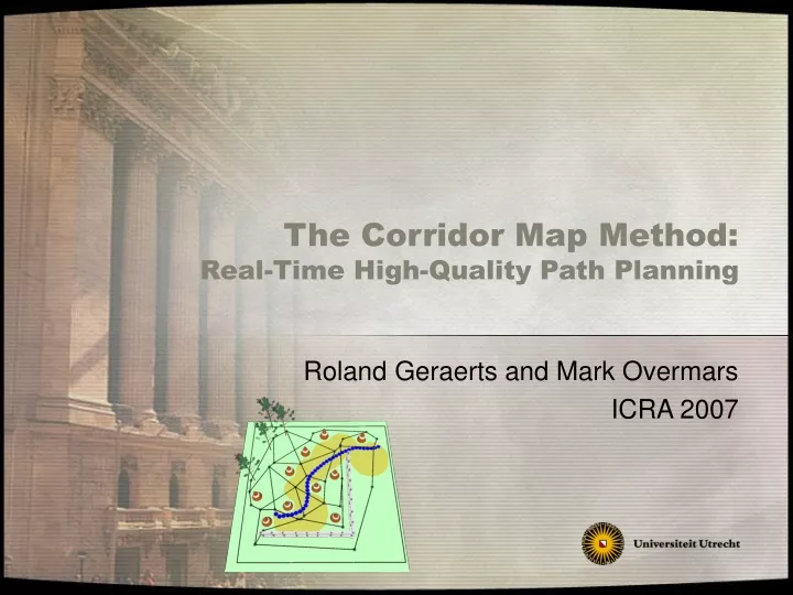
The Corridor Map Method:Real-Time High-Quality Path Planning Roland Geraerts and Mark Overmars ICRA 2007
Previous work • Potential field planners • Flexible • Slow / local minima • Probabilistic Roadmap Methods • Fast • Ugly paths • Output: fixed paths in response to a query • Predictable motions • Lacks flexibility when environment changes
Our planner • Requirements • High-quality paths • Flexible • Extremely fast • Current limitations • The robot is modeled by a disc • Experiments with only 2D problems
The Corridor Map Method • Construction phase (off-line) • Create a system of collision-free corridors for the static obstacles Graph Corridor map: graph + clearance
Query Corridor: backbone path + clearance Path The Corridor Map Method • Query phase (on-line) • Extract corridor for given start and goal • Extract path by following attraction point
r g α(x) d x The Corridor Map Method • Attraction point α(x) • Robot’s location: x • Robot’s goal: g • Radius circle: r • Euclidean distance: d • Path is obtained by integration over time while updating the velocity, position, and attraction point of the robot • For other behavior: locally adjust robot’s path by adding forces
Adding forces For each obstacle, add repulsive force to the robot Creating a sub-corridor For each obstacle, move backbone path locally and recompute clearance info Avoiding obstacles
α(x, 0.00) α(x, 0.05) α(x, 0.10) α(x, 0.25) Creating shorter paths • Attraction point α(x) corresponds to point B[t] on the backbone path • Add additional valid attraction point α(x, Δt), corresponding to point B[t + Δt] • Valid means: x can see point B[t + Δt]
Experimental setup • Single path planning system • Created in Visual C++, Windows XP • 2.66 GHz P4 processor, 1 GB memory • Each experiment was run 100 times • Statistics: running time of query phase, CPU load • Input graphs created using • “Creating High-quality Roadmaps for Motion Planning in Virtual Environments“-IROS 2006 • Environments were discretized: 100x100 cells
Maze Field Experimental setup 1.6 seconds 20 seconds
Maze Query time: 2.41 ms CPU load: 0.026% Field Query time: 0.84 ms CPU load: 0.029% Experiments – Smooth paths
Maze: adding forces Query time: 7.0—9.0 ms CPU load: 0.05—0.06% Maze: sub-corridor Query time: 3.0—13.6 ms CPU load: 0.025—0.10% Experiments – Obstacles
Maze Experiments – Obstacles
Field: adding forces Query time: 2.0—2.3 ms CPU load: 0.05—0.05% Field: sub-corridor Query time: 1.0—7.0 ms CPU load: 0.03—0.16% Experiments – Obstacles
Field Experiments – Obstacles
Maze: Δt = 0 Query time: 2.41 ms CPU load: 0.026% Maze: Δt = 0.2 Query time: 9.64 ms CPU load: 0.104% Experiments – Short paths
Maze Experiments – Short paths
Field: Δt = 0 Query time: 0.84 ms CPU load: 0.029% Field: Δt = 0.2 Query time: 3.36 ms CPU load: 0.116% Experiments – Short paths
Field Experiments – Short paths
Conclusions • The CMM produces high-quality paths • Natural paths: smooth, short / large clearance • The CMM is flexible • Paths are locally adjustable • The CMM is fast • CPU load < 0.1%
Future work • Extend experimentswith 2½D / 3D problems • Study applications • Planning of a group • Steering a camera • Alternative routes • Tactical planning