Download
1 / 12
140 likes | 308 Vues
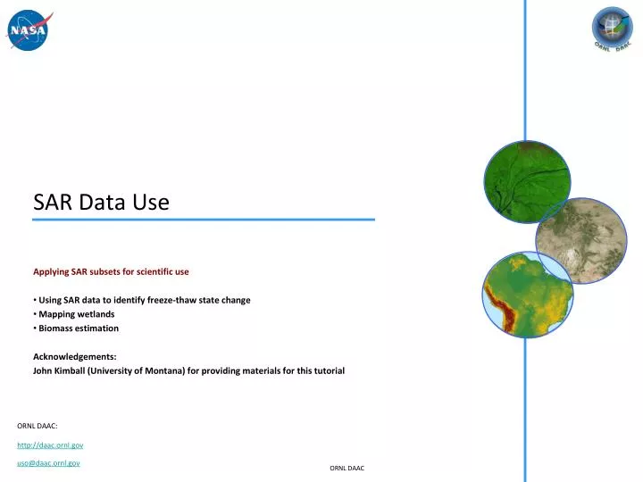
SAR Data Use. Applying SAR subsets for scientific use Using SAR data to identify freeze-thaw state change Mapping wetlands Biomass estimation Acknowledgements: John Kimball (University of Montana) for providing materials for this tutorial.

E N D
SAR Data Use Applying SAR subsets for scientific use Using SAR data to identify freeze-thaw state change Mapping wetlands Biomass estimation Acknowledgements: John Kimball (University of Montana) for providing materials for this tutorial
Mapping Freeze-Thaw state : Why is it important? http://freezethaw.ntsg.umt.edu/ Major landscape hydrological processes embracing the remotely sensed freeze/thaw signal include • Timing and spatial dynamics of seasonal snowmelt • Associated soil thaw due to snowmelt • Runoff generation • Flooding • Ice breakup in large rivers andlakes • Timing and length of vegetation growing seasons and associated productivity and trace gas exchange. Source: McDonald, K. C. and Kimball, J. S. 2006. Estimation of Surface Freeze–Thaw States Using Microwave Sensors. Encyclopedia of Hydrological Sciences. 1
Using SAR data to identify freeze-thaw state change The basis of the RADAR remote sensing based freeze-thaw measurement is the large shift in dielectric constant and associated backscatter as the landscape shifts between predominantly frozen and thawed conditions. The figure on the right shows the large L-band dB shift during a freeze-thaw transition event as captured from multi-temporal AIRSAR acquisitions. Way, J.B. et al., 1994. Trans. Geosci. Rem. Sens. 32, 2. • Bonanza Creek, AK http://www.lter.uaf.edu/ 2
Dielectric constant for liquid water and ice L-band (Real Part) S-band (Imaginary Part) ku-band Dielectric Constant C-band 1 10 100 Frequency (GHz) • The dielectric constant of liquid water and ice as a function of frequency across the microwave spectrum; the Dielectric constant of liquid water varies with frequency, whereas that of pure ice is constant and low (Ulaby, et al., 1986, p. 848; Kraszewski, 1996). 3
Time-Series L-band Classification of Freeze-Thaw Temporal change classification of landscape freeze-thaw status using JERS-1 L-band radar backscatter series over Bonanza Creek AK. The JERS-1 SAR data is aggregated to 100 m spatial resolution. The sequence of image windows are 25 km x 25 km in extent, which is equivalent to 1 satellite footprint from AMSRE or SSM/I. The resulting freeze-thaw classifications are compared against in situ measurements of vegetation canopy stem temperatures. The sequence of SAR scenes show a ~3dB shift in L-band backscatter between frozen and non-frozen conditions. (from McDonald and Kimball, EHS 2005). 4
Open Water mapping using L-Band RADAR:Importance of Mapping wetlands Wetlands play a critical role in regulating the movement of water within watersheds as well as in the global water cycle (Richardson 1994; Mitsch and Gosselink 1993). Wetlands act as major sinks and sources of important atmospheric greenhouse gases and can switch between atmospheric sink and source in response to climatic and anthropogenic forces in ways that are poorly understood. Despite their importance in the carbon cycle, the locations, types, and extents of northern wetlands are not accurately known. (J. Whitcomb et al. 2009. Can. J. Rem. Sens. 35, 54-72). Many plant, fish, bird, reptile, and amphibians rely on wetlands for their habitat. Wetlands play a critical role in nutrient cycling. Used for recreation. 5
Wetlands Mapping Map of open water area of Alaska’s North Slope and detailed view of the Kuparuk River Basin derived from JERS-1 SAR L-band data. Blue represents open water. The SAR mosaic of Alaska was assembled from imagery collected during mid-summer of 1998. (J. Whitcomb et al. 2009. Can. J. Rem. Sens. 35, 54-72). 6
Wetlands classification using SAR data Classified high-water (inundation) mosaic derived from L-band SAR imagery from JERS-1 for the Cabaliana floodplain along the Solimoes river, Amazonas, Brazil. Classes are open water (blue), flooded forest (white), flooded herbaceous (floating meadows; magenta), flooded woodland (tan), non-flooded forest (green), and non-wetland (black). Source: Lowry J, Hess L & Rosenqvist A 2009. Mapping and monitoring wetlands around the world using ALOS PALSAR: the ALOS Kyoto and Carbon Initiative wetland products. In Lecture Notes in Geoinformation and Cartography - Innovations in Remote Sensing and Photogrammetry, eds. S Jones & K Reinke. Springer-Verlag, Berlin, 105-120. 7
Biomass estimation: Applications • Carbon accounting • Green house gas source/sink estimates • Climate change studies • Policy decisions Relationships between backscattering coefficient and above-ground biomass density. Source: http://www.eci.ox.ac.uk/research/biodiversity/linkcarbon.php 8
Biomass estimation (1/2) LAI (projected) Stem Biomass (Mg C ha-1) 1:1 1:1 AIRSAR 3x3 Window AIRSAR 3x3 Window Biomass Harvest Plot Scatterplots of AIRSAR vs. biomass harvest plot stem biomass (Mg C ha-1) and LAI (defined as 50% of total LAI) estimates for 1994 within the BOREAS Southern Study Area (SSA). The AIRSAR results were obtained by extracting mean, maximum and minimum values from 3x3 pixel windows centered over approximately 13 tower sites, carbon evaluation and auxiliary harvest plot locations within the SSA. Biomass sampling within each plot was structured to characterize vegetation within an approximate 30 x 30 m area from a network of 1 – 4 replicate plots ranging in size from 56 m2 to 900 m2 depending on tree densities (Gower et al. 1997). Grey lines depict the ranges (Max. - Min.) of values reported within AIRSAR and harvest plot windows (Kimball et al. 2000. Tree Physiology 20(11)). Kimball et al. 2000. Tree Phys 20(11), 761-775. 9 Biomass Harvest Plot
Biomass estimation (2/2) ALOS PALSAR L-band HH (a) and HV (b) radar backscatter plotted against field-measured above-ground biomass (AGB, Mg ha-1) for four combined sites in central Africa representing tropical savanna and woodland types in Camaroon, Uganda and Mozambique; x-axes are shown with conventional log10 scales. Second order log regression lines are fitted. The relationships were highly significant, similar among sites, and displayed high prediction accuracies up to 150 Mg ha-1 (+/-20%). From Mitchard et al. 2009. Geophys Res. Lett 36, L23401. Mitchard et al. 2000. Geophys. Res. Lett. 36. 10
Mapping land cover Map of land cover types of the Amazon basin obtained from JERS-1 L-band SAR mosaic and texture measures. The map includes 14 cover types identified in the legend (Saatchi et al. 2000. Int. J. Remote Sensing 21(6-7), 1201-1234). Saatchi et al. 2000. Int. J. Rem. Sens. 21(6-7). 11