Download
1 / 35
350 likes | 475 Vues
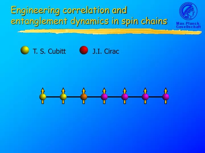
T. S. Cubitt. J.I. Cirac. Engineering correlation and entanglement dynamics in spin chains. T. S. Cubitt. Motivation and goals Time evolution of a chain Correlation and entanglement wave-packets Engineering the dynamics: solitons etc. Fermionic gaussian state formalism Conclusions.

E N D
T. S. Cubitt J.I. Cirac Engineering correlation and entanglement dynamics in spin chains
T. S. Cubitt • Motivation and goals • Time evolution of a chain • Correlation and entanglement wave-packets • Engineering the dynamics: solitons etc. • Fermionic gaussian state formalism • Conclusions Engineering correlation and entanglement dynamics in spin chains J.I. Cirac
Many papers on correlations/entanglement of ground states • Fewer on time-dependent behaviour away from equilibrium • New experiments… • …motivate new theoretical studies of non-equilibrium behaviour. Conceptual motivation: new experiments
Many papers on correlations/entanglement of ground states. • Fewer on time-dependent behaviour away from equilibrium • In Phys. Rev. A 71, 052308 (2005), we used our entanglement rate equations to bound the time taken to entangle the ends of a length L chain. • Left open question of whether our pL lower bound is tight. • In J.Stat.Mech. 0504 (2005) p.010, Calabrese and Cardy investigated the time-evolution of block-entropy in spin chains. • Bravyi, Hastings and Verstraete (quant-ph/0603121)recently used Lieb-Robinson to prove tighter, linear bound. Existing results
“Traditional” solution to entanglement distribution:build a quantum repeater. • Getting to the ground state may be unrealistic. • Why not use non-equilibrium dynamics to distribute entanglement? • But a real quantum repeater involves particle interactions, e.g. atoms in cavities. • Alternative (e.g. Popp et al., Phys. Rev. A 71, 042306 (2005)): use entanglement in ground state: Practical motivation: quantum repeaters
T. S. Cubitt J.I. Cirac • Motivation and goals • Time evolution of a chain • Correlation and entanglement wave-packets • Engineering the dynamics: solitons etc. • Fermionic gaussian state formalism • Conclusions Engineering correlation and entanglement dynamics in spin chains
As an exactly-solvable example, we take the XY model… anisotropy magnetic field …and start it in some separable state, e.g. all spins +. Time evolution of a spin chain (1)
Fourier: • Solved by a well-known sequence of transformations: • Bogoliubov: • Jordan-Wigner: Time evolution of a spin chain (2)
Initial state N|+i… …is vacuum of the cl=zj-l operators. • Wick’s theorem: all correlation functions hxm…pni of the ground state of a free-fermion theory can be re-expressed in terms of two-point correlation functions. • Our initial state is a fermionic Gaussian state: it is fully specified by its covariance matrix: Time evolution of a spin chain (3)
Hamiltonian… …is quadratic in x and p. Gaussian state stays gaussian under gaussian evolution. • From Heisenberg equations, can show that time evolution under any quadratic Hamiltonian: corresponds to an orthogonal transformation of the covariance matrix: Time evolution of a spin chain (4)
Initial state is a fermionic gaussianstate in xl and pl. • Time-evolution is a fermionic gaussianoperation in xk and pk. • Fourier and Bogoliubov transformations are gaussian: Connected by Fourier and Bogoliubov transformations Time evolution of a spin chain (5)
xk , pk xk , pk xk , pk xk , pk xk , pkxl , pl time-evolve initial state • Putting everything together: Time evolution of a spin chain (phew!)
T. S. Cubitt J.I. Cirac • Motivation and goals • Time evolution of a chain • Correlation and entanglement wave-packets • Engineering the dynamics: solitons etc. • Fermionic gaussian state formalism • Conclusions Engineering correlation and entanglement dynamics in spin chains
We can get string correlationshanzlbmifor free… • Equations are very familiar: wave-packets with envelopeS propagating according to dispersion relation(). • Given directly by covariance matrixelements, e.g.: String correlations
Two-point connected correlation functions hznzmi - hznihzmi can also be obtained from the covariance matrix. • Again get wave-packets (3 of them) propagating according to dispersion relation(k). • Using Wick’s theorem: Two-point correlations
The relevant measure for entanglement distribution (e.g. in quantum repeaters) is the localisable entanglement (LE). • Definition: maximum entanglement between two sites (spins) attainable by LOCC on all other sites, averaged over measurement outcomes. • As with all operationally defined entanglement measures, LE is difficult to calculate in practice. • Best we can hope for is a lower bound. • Popp et al., Phys. Rev. A 71, 042306 (2005): LE is lower-bounded by any two-point connected correlation function. • In case you missed it: we’ve just calculated this! What about entanglement?
T. S. Cubitt J.I. Cirac • Motivation and goals • Time evolution of a chain • Correlation and entanglement wave-packets • Engineering the dynamics: solitons etc. • Fermionic gaussian state formalism • Conclusions Engineering correlation and entanglement dynamics in spin chains
In particular, around =1.1, =2.0 all three wave-packets in the two-point correlation equations are nearly identical • !localised packets propagate at well-defined velocity with minimaldispersion: “soliton-like” behaviour • In other parameter regimes: narrower wave-packets in nearly linear regions of dispersion relation • ! packets maintain their coherence as they propagate • In some parameter regimes: broadwave-packets and a highly non-linear dispersion relation • ! correlations rapidly disperse and disappear Correlation wave-packets
The system parameters and simultaneously control both the dispersion relation and form of the wave-packets. • In some parameter regimes: broadwave-packets and a highly non-linear dispersion relation • ! correlations rapidly disperse and disappear: (=10, =2) Correlation wave-packets (1)
In other parameter regimes, all three wave-packets in the two-point correlation equations are nearly identical • !localised packets propagate at well-defined velocity with minimaldispersion: “soliton-like” behaviour: (=1.1, =2) Correlation/entanglement solitons
If the parameters are changed with time, • ! Effective evolution under time-averaged Hamiltonian. • In general, time-ordering is essential. • But if parameters change slowly, dropping it gives reasonable approximation. • If we stay within “soliton” regime, adjusting the parameters only changes gradient of the dispersion relation, without significantly affecting its curvature. • ! Can speed up and slow down the “solitons”. Controlling the soliton velocity (1)
Starting from =1.1, =2.0 and changing at rate +0.01: Controlling the soliton velocity (2)
What happens if we do the opposite: rapidly change parameters from one regime to another? • Can calculate this analytically using same machinery as before. • Resulting equations are uglier, but still separate into terms describing multiple wave-packets propagating and interfering. Get four types of behaviour for the wave-packets: • Evolution according to 1 for t1, then 2 • Evolution according to 1 for t1, then -2 • Evolution according to 1untilt1, no evolution thereafter • Evolution according to 2starting att1 • Choose parameters so that “frozen” packets remain relatively coherent, whilst others rapidly disperse. “Quenching” correlations (1)
Choose parameters so that “frozen” packets remain relatively coherent, whilst others rapidly disperse. • ! can move correlations/entanglement to desired location, then “quench” system to freeze it there. • E.g. =0.9, =0.5 changed to =0.1, =10.0 at t1=20.0: “Quenching” correlations (2)
T. S. Cubitt J.I. Cirac • Motivation and goals • Time evolution of a chain • Correlation and entanglement wave-packets • Engineering the dynamics: solitons etc. • Fermionic gaussian state formalism • Conclusions Engineering correlation and entanglement dynamics in spin chains
There is another LE bound we can calculate… • Not a covariance matrix element because of |*i. • Recall concurrence: • Localisable concurrence: What about entanglement? (2)
Recap of gaussian state formalism… • What’s missing? A fermionicphase-space representation. Bosonic case Fermionic case • Operators a, aycommute • Operators c, cyanti-commute • States specified by symmetric covariance matrix • States specified by antisymmetric covariance matrix • Gaussian operations $symplectic transformations of • Gaussian operations $orthogonal transformations of Fermionic gaussian formalism
For bosons… • Eigenstates of an are coherent states: an|i = n|i • Define displacement operators: D()|vaci = |i • Characteristic function for state is:() = tr(D() ) For fermions… • Try to define coherent states: cn|i = n|i… • …but hit up against anti-commutation:cncm|i = m n|i but cncm|i = -cmcn|i = -n m|i • Define gaussian state to have gaussian characteristic function: • Eigenvalues anti-commute!? Fermionic phase space (1)
Coherent states and displacement operators now work:cncm|i = -cmcn|i = -n m|i = m n|i = cncm|i • Characteristic function for a gaussian state is again gaussian: • Grassman calculus: • Solution: expand fermionic Fock space algebra to include anti-commuting numbers, or “Grassmann numbers”, n. • Grassman algebra:n m = -m n)n2=0; for convenience n cm = -cm n Fermionic phase space (2)
We will need another phase-space representation: the fermionic analogue of the P-representation. • Essentially, it is a (Grassmannian) Fourier transform of the characteristic function. • Useful because it allows us to write state in terms of coherent states: • For gaussian states: Fermionic phase space (3)
Finally, • Recall bound on localisable entanglement: • Substituting the P-representation for states and * :and expanding xnand pn in terms of cnand cn y, the calculation becomes simple since coherent states are eigenstates of c. • Not very useful since bound 0 in thermodynamic limit N 1. What about entanglement (3)
Already leading to new theoretical results, e.g.: • Michael Wolf has used fermionic gaussian states to prove an area law for a large class of fermionic systems, in arbitrary dimensions: Phys. Rev. Lett. 96, 010404 (2006) • However, experimentalists are starting to build atomic analogues of quantum optical setups: e.g. atom lasers, atom beam splitters. • Fermionic gaussian state formalism may become important as fermionic gaussian states and operations move into the lab. Fermionic phase space (4)
T. S. Cubitt J.I. Cirac • Motivation and goals • Time evolution of a chain • Correlation and entanglement wave-packets • Engineering the dynamics: solitons etc. • Fermionic gaussian state formalism • Conclusions Entanglement flow in multipartite systems
Have shown that correlation and entanglement dynamics in a spin chain can be described by simple physics: wave-packets. Correlation dynamics can be engineered: • Set parameters to produce “soliton-like” behaviour • Control “soliton” velocity by adjusting parameters slowly in time • Freeze correlations at desired location by quenching the system • Developed fermionic gaussian state formalism, likely to become more important as experimentalists are starting to do gaussian operations on atoms in the lab (atom lasers, atomic beam-splitters…). Conclusions