Download
1 / 18
200 likes | 234 Vues
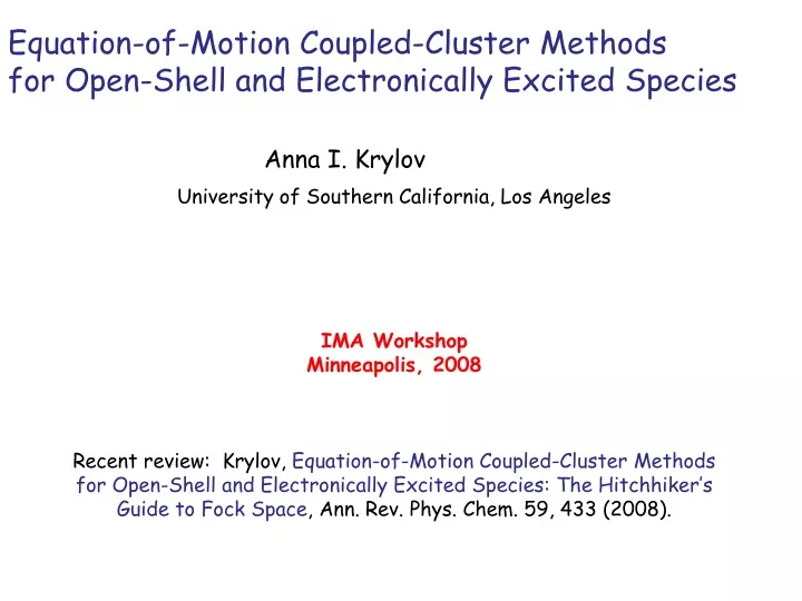
Equation-of-Motion Coupled-Cluster Methods for Open-Shell and Electronically Excited Species. Anna I. Krylov. University of Southern California, Los Angeles IMA Workshop Minneapolis, 2008 Recent review: Krylov , Equation-of-Motion Coupled-Cluster Methods

E N D
Equation-of-Motion Coupled-Cluster Methods for Open-Shell and Electronically Excited Species Anna I. Krylov University of Southern California, Los Angeles IMA Workshop Minneapolis, 2008 Recent review: Krylov, Equation-of-Motion Coupled-Cluster Methods for Open-Shell and Electronically Excited Species: The Hitchhiker’s Guide to Fock Space, Ann. Rev. Phys. Chem. 59, 433 (2008).
Outline: • CI and truncated CI: overview. • Size-extensive alternative: Coupled-cluster ansatz. • 3. Extension to electronically excited and open-shell states: • EOM-CC formalism. • 4. EOM-CC advantages and limitations. • 5. Examples. • 6. More rigorous derivation of EOM-CC equation.
Exact solution of the Schroedinger equation and configuration • interaction (CI) approach • Chose one-electron basis set (M orbitals), construct reference determinant • (N orbitals) F0 • 2. Linear ansatz for the wave-function: Y=(1+C1+C2+ … CN)F0, where C1=Sciaa+i • Thus, operators C1..CN will generate all possible distributions of N electrons over • M orbitals • 3. Energy functional: E=<Y|H|Y>/<Y|Y> • Amplitude equations: Variational Principle -> • CI eigen-problem for the ground and excited states: HC=CE • Exact solution (FCI). Approximations: truncated CI • Hierarchy of approximations: HF->CISD->CISDT->….->FCI • Problems with truncated CI: violation of size extensivity • For non-interacting systems (HAB=HA+HB): EAB=EA+EB and YAB=YAxYB • But: YACISDxYBCISD is not equal YABCISD
Solution: Coupled-cluster ansatz: • Y=eTF0=(1+T + ½T2 + 1/6 T3 + … ) F0, T1=Stiaa+i • If T=T1+T2 : • - higher-order excitations are present, e.g., (T1)2, (T2)2, • (T2)2T1, etc • - size-extensivity is satisfied: • eTAxeTB=eTA+TB (provided that T is strictly an excitation • operator wrt the reference vacuum); • but exponential expansion does not terminate in energy • functional E=<Y|H|Y>/<Y|Y> for variational principle. • Equations (projection principle): E=<F0|e-T H eT | F0> • <Fm|e-T H eT -E| F0>=0 • Can be recast in a more general variational form and • extended to excited states.
Hierarchy of approximations to the exact wave function: Single-reference models for the ground state SCF : Y=F0=|j1...jn> Yex=R1Y0(CIS) MP2 : SCF + T2by PT CIS + R2 by PT [CIS(D)] CCSD: Y=exp(T1+T2) F0 Yex=(R1+R2)Y0(EOM-CCSD) CCSD(T): CCSD + T3 by PT CCSDT: Y=exp(T1+T2+T3) F0 Yex=(R1+R2+R3)Y0(EOM-CCSDT) …………………………………………………................................. FCI: Y=(1+T1+T2 + … +Tn )F0 - exact! T2F0 F0 T1F0 T2=0.25*Sijab tijab a+b+ ji T1=Sia tia a+ j
Why open shells and electronically excited states are difficult? Electronic degeneracy -> multi-configurational wavefunctions The CC hierarchy of approximations breaks down.
Equation-of-motion theory and specific models: Rowe, Rev. Mod. Phys. 40, 153 (1968) Simons, Smith, JCP 58, 4899 (1973) McWeeny, “Methods of Molecular Quantum Mechanics” Lowdin, “Some aspects of the Hamiltonian and Liouvillian Formalism …”, AQC 17, 285 (1985) Sekino, Bartlett, IJQCS 18 255 (1984) Stanton, Bartlett, JCP 98, 7029 (1993) Stanton, Gauss, JCP 101, 8938 (1994) Nooijen, Bartlett, JCP 102, 3629 (1995) Wladyslawski, Nooijen, ACS series 828, 65 (2002) Also works of Mukherjee, Pal, Piecuch, Emrich, McKoy, Kutzelnigg, Kaldor, Werner, Hirata. Related: linear response works of Koch, Jorgen, Jensen, Jorgensen, Head-Gordon, Lee, Korona, etc. SAC-CI by Nakatsuji. Recent developments: Crawford, Piecuch, Kowalsky. AND MUCH MORE!!! Recent review: Krylov, Equation-of-Motion Coupled-Cluster Methods for Open-Shell and Electronically Excited Species: The Hitchhiker’s Guide to Fock Space, Ann. Rev. Phys. Chem. 59, 433 (2008).
Equation-of-Motion Coupled-Cluster Methods 1. regardless of T, has same spectrum as H 2. Y=F0 + R1F0 + R2F0 + ......, where Rn is some general excitation operator, e.g., R1=Sria a+i (or R1=Sra a+or R1=Srii, etc) 3. Apply bi-Variational Principle: EOM eigen-problem 4. Specific EOM model: choice of excitation operators T, R, and the reference F0
EOM models: Choice of T 1. Excitation level, e.g., T=T1+T2 2. Amplitude equations. If T satisfies CC equations, F0F1 F2 F0F1 F2 - size extensivity - compact wf-s, e.g., Yexact=F0 - correlation effects are "wrapped in": same scaling but higher accuracy
EOM MODELS: CHOICE OF R and F0 Yijab Y0 Yia EOM-EE:Y(Ms=0) =R(Ms=0)Y0(Ms=0) EOM-IP:Y(N) =R(-1)Y0(N+1) Y0 Yi Yija EOM-EA:Y(N) =R(+1)Y0(N-1) Y0 Ya Yiab EOM-SF:Y(Ms=0)=R(Ms=-1)Y0(Ms=1) Y0 Yia
Size-extensivity: Be example Be /6-31G* Be @ USC & Ne @ Berkeley Krylov, CPL 350, 522 (2001); Sears, Sherrill, Krylov, JCP, 118, 9084 (2003)
Equation-of-Motion Coupled-Cluster Theory Truncated EOM model, e.g., EOM-CCSD: diagonalize H-bar in the basis of singly and doubly excited determinants (amplitudes T - from CCSD equations). Same cost as CISD (N6) but: - size-intensive - has higher accuracy (correlation is “wrapped in” through the similarity transformation). Multistate method, describes degeneracies and near-degeneracies, as well as interacting states of different nature (just because it is diagonalization problem). Bi-variational formulation facilitates properties calculations (Hellmann-Feynman theorem).
Limitations of CCSD and EOM-CCSD: • Scaling is N6. • 2. Need triples corrections for “chemical accuracy”, e.g. • CCSD(T) (scales N7). • 3. Not always possible to find a well-behaved reference from • which target states of interest can be accessed via single • excitations -> cannot describe global potential energy • surfaces. • 4. Non-hermitian nature sometimes causes problems (e.g., • wrong dimensionality of conical intersections).
Excited states of sym-triazine p*n manifold p*p manifold Rsn manifold Rpn manifold • - All low-lying excited states of Tz involve transitions from/to degenerate MOs. • Some are Jahn-Teller distorted and some exhibit glancing-like intersections. • EOM-EE describes accurately these manifolds, interactions, and degeneracies. Mozhayskiy, Babikov, and Krylov, JCP 124, 224309 (2006) Schuurman and Yarkony, JCP 126, 044104 (2007)
Excited singlet states of sym-triazine Neutral geometry Cation geometry EOM-CCSD/6-311++G**
Cs · · Tz+ Cs+··Tz* EOM for the [Cs..Tz]+ complex EOM reference: [Cs+..Tz] Initial charge transfer state Single excitations of the reference state Initial CT state Final charge transfer states Single excitations of initial CT state Double excitations of initial CT state
Equation-of-motion formalism Consider the Hamiltonian H (non-hermitian), and its exact eigenstates |0> & |f>: H|0>=E0|0> & H|f>=Ef|f> Consider excitation operator R(f): R(f)|0> =|f> Define R(f) as: R(f)=|f><0| For any |0> (<0|0> non-zero): R(f)|0>=|f><0|0> => [H,R(f)]|0> = wof R(f)|0> (*) - no knowledge of exact initial and final states is necessary to determine exact wof - (*) is an operator equation, valid not only in a subspace. Define de-excitation operator L(f): L(f)=|0><f| EOM functionals: wof=<0|L(f)[H,R(f)]|0> / <0|L(f)R(f)|0> wof=<0|[L(f),[H,R(f)]]-|0> / <0|[L(f),R(f)]-|0> wof=<0|[L(f),[H,R(f)]]+|0> / <0|[L(f),R(f)]+|0> ALL three functionals: - exact result when R, L is expanded over the complete basis set - identical equations when the killer condition is satisfied: L(f) |0> = 0 (reference is “true” vacuum) or L(f) |0> = |0><f|0> = 0 (reference is orthogonal to final states)
EOM equations 1. Expand R, L over a finite operator basis set: R(f) = Sk rkrk L(f)=Sk lklk 2. Use bivariational priciple with any of the three funcionals, arrive to the matrix equations: (H-E0)R=RW L(H-E0)=WL E0=<0|H|0>