Download
1 / 54
540 likes | 546 Vues
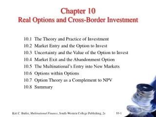
Chapter 18 Real Options and Cross-Border Investment. 18.1 Types of Options 18.2 The Theory and Practice of Investment 18.3 Puzzle #1: Market Entry and the Option to Invest 18.4 Uncertainty and the Value of the Option to Invest 18.5 Puzzle #2: Market Exit and the Abandonment Option

E N D
Chapter 18Real Options and Cross-Border Investment 18.1Typesof Options 18.2The Theory and Practice of Investment 18.3 Puzzle #1: Market Entry and the Option to Invest 18.4Uncertainty and the Value of the Option to Invest 18.5 Puzzle #2: Market Exit and the Abandonment Option 18.6 Puzzle #3: The Multinational’sEntry into New Markets 18.7 Real Options as a Complement to NPV 18.8 Summary
Options on real assets • A real option is an option on a real asset • Real options derive their value from managerial flexibility • Option to invest or abandon • Option to expand or contract • Option to speed up or defer
Options on real assets • Simple options • European - Exercisable at maturity • American - Exercisable prior to maturity • Compound option • An option on an option • Switching option - An alternating sequence of calls and puts • Rainbow option • Multiple sources of uncertainty
Two types of options • Call option An option to buy an asset at a pre-determined amount called the exercise price • Put option An option to sell an asset
The conventionaltheory of investment Discount expected future cash flows at an appropriate risk-adjusted discount rate NPV = St [E[CFt] / (1+i)t] • Include only incremental cash flows • Include all opportunity costs
Three investment puzzles • MNC’s use of inflated hurdle rates in uncertain investment environments • MNC’s failure to abandon unprofitable investments • MNC’s negative-NPVinvestments in new or emerging markets
Puzzle #1Firms’ use of inflated hurdle rates Market entry and the option to invest • Investing today means foregoing the opportunity to invest at some future date, so that projects must be compared against similar future projects • Because of the value of waiting for more information, corporate hurdle rates on investments in uncertain environments are often set above investors’ required return
An example of the option to invest • Investment I0 = PV(I1) = $20 million The present value of investment is assumed to be $20 million regardless of when investment is made. • Price of oil P = $10 or $30 with equal probability Þ E[P] = $20 • Variable production cost V = $8 per barrel • E[production] = Q = 200,000 barrels/year • Discount rate i = 10%
The option to invest asa now-or-never decision NPV(invest today) = ($20-$8) (200,000) / .1 - $20 million = $4 million > $0 Þinvest today(?)
The option to wait one yearbefore deciding to invest NPV = [ (E[P]-V) Q / i ] / (1+i) - I0 In this example, waiting one year reveals the future price of oil
The investment timing option NPV(wait 1 year½P=$30) = (($30-$8)(200,000) /.1) / (1.1) - $20,000,000 = $20,000,000 > $0 Þ invest if P = $30 NPV(wait 1 year½P=$10) = (($10-$8)(200,000) /.1) / (1.1) - $20,000,000 = -$16,363,636 < $0 Þ do not invest if P = $10 Þ NPV(wait 1 year½P=$10) = $0
The investment timing option NPV(wait 1 year) = Probability(P=$10) (NPV$10) + Probability(P=$30) (NPV$30) = ½ ($0) + ½ ($20,000,000) = $10,000,000 > $0 Þ wait one year before deciding to invest
Option value = intrinsic + time values Intrinsic value = value if exercised immediately Time value = additional value if left unexercised
The opportunity cost of investing today Option Value = Intrinsic Value + Time Value NPV(wait 1 year) = Value if exercised + Additional value immediatelyfrom waiting $10,000,000 = $4,000,000 + $6,000,000
A resolution of Puzzle #1Use of inflated hurdle rates Managers facing this type of uncertainty have four choices • Ignore the timing option (?!) • Estimate the value of the timing option using option pricing methods • Adjust the cash flows with a decision tree that captures as many future states of the world as possible • Inflate the hurdle rate (apply a “fudge factor”) to compensate for high uncertainty
The value of BP’s 25 option to invest 20 15 10 Time value 5 0 0 5 10 15 20 25 30 35 40 Value of an oil well Option value = intrinsic + time values Option value Intrinsic value
Call option value determinants Relation to call option BP Option value determinant value example Value of the underlying asset P + $24 million Exercise price of the option K - $20 million Volatility of the underlying asset sP+ ($3.6m or $40m) Time to expiration of the option T + 1 year Riskfree rate of interest RF + 10% Time value = f ( P, K, T,sP, RF )
Volatility and option value Option value Exercise price Value of the underlying asset
Exogenous price uncertainty Exogenous uncertainty is outside the influence or control of the firm Oil price example P1 = $35 or $5 with equal probability Þ E[P1] = $20/bbl NPV(invest today) = (($20-$8)(200,000) /.1) - $20 million = $4,000,000 > $0 Þinvest today?
Exogenous price uncertainty NPV(wait 1 year½P1=$35) = (($35-$8)200,000 /.1)/1.1 - $20 million = $29,090,909 > $0 Þ invest if P1=$35 NPV(wait 1 year½P1=$5) = (($5-$8)(200,000) /.1)/1.1 - $20 million = -$25,454,545 < $0 Þ do not invest if P1=$5
Exogenous price uncertainty NPV(wait one year) = (½)($0)+(½)($29,090,909) = $14,545,455 > $0 Þ wait one year before deciding to invest
Time value & exogenous uncertainty Option value = Intrinsic value + Time value ±$10 $10,000,000 = $4,000,000 + $6,000,000 ±$15 $14,545,455 = $4,000,000 + $10,545,455 The time value of an investment option increases with exogenous price uncertainty
Puzzle #2Failure to abandon losing ventures Market exit & the option to abandon • Abandoning today means foregoing the opportunity to abandon at some future date, so that abandonment today must be compared to future abandonment • Because of the value of waiting for additional information, corporate hurdle rates on abandonment decisions are often set above investors’ required return
An example of the option to abandon • Cost of disinvestment I0 = PV(I1) = $2 million • Price of oil P = $5 or $15 with equal probability Þ E[P] = $10 • Variable production cost V = $12 per barrel • E[production] = Q = 200,000 barrels/year • Discount rate i = 10%
The option to abandon asa now-or-never decision NPV(abandon today) = -($10-$12) (200,000) / .1 - $2 million = $2 million > $0 Þabandon today(?)
The abandonment timing option NPV(wait 1 year½P=$5) = -(($5-$12)(200,000) /.1) / (1.1) - $2 million = $10,727,273 > $0 Þabandon if P=$5 NPV(wait 1 year½P=$15) = -(($15-$12)(200,000) /.1) / (1.1) - $2 million = -$7,454,545 < $0 Þdo not abandon if P=$15
The abandonment timing option NPV(wait 1 year) = Probability(P=$5) (NPV$5) + Probability(P=$15) (NPV$15) = ½ ($10,727,273) + ½ ($0) = $5,363,636 > $0 Þ wait one year before deciding to abandon
Opportunity cost of abandoning today Option Value =Intrinsic Value+ Time Value NPV(wait 1 year) = NPV(abandon today) + Additional value from waiting 1 year $5,363,636 = $2,000,000 + $3,363,636
Hysteresis Cross-border investments often have different entry and exit thresholds • Cross-border investments may not be undertaken until the expected return is well above the required return • Once invested, cross-border investments may be left in place well after they have turned unprofitable
Puzzle #3Negative-NPV entryinto emerging markets • Firms often make investments into emerging markets even though investment does not seem warranted according to the NPV decision rule • An exploratory (perhaps negative-NPV) investment can reveal information about the value of subsequent investments
Growth options and project value VAsset = VAsset-in-place + VGrowth options
Consider a negative-NPV investment • Initial investment I0 = PV(I1) = $20 million • Price of Oil P = $10 or $30 with equal probability Þ E[P] = $20 • Variable production cost V = $12 per barrel • E[production] = Q = 200,000 barrels/year • Discount rate i = 10%
The option to invest asa now-or-never decision NPV(invest today) = ($20-$12) (200,000)/.1 - $20,000,000 = -$4 million < $0 Þ do not invest today(?)
Endogenous price uncertainty • Uncertainty is endogenous when the act of investing reveals information about the value of an investment • Suppose this oil well is the first of ten identical wells that BP might drill • and that the quality and hence price of oil from these wells cannot be revealed without drilling a well
Invest today in order to reveal information about future investments Investing today E[P] = $20/bbl P = $30/bbl reveals information P = $10/bbl
The investment timing option NPV(wait 1 year½P=$30) = (($30-$12)(200,000) /.1) / (1.1) - $20,000,000 = $12,727,273 > $0 Þinvest if P = $30 NPV(wait 1 year½P=$10) = (($10-$12)(200,000) /.1) / (1.1) - $20,000,000 = -$53,272,727 < $0 Þdo not invest if P = $10
A compound option in the presence of endogenous uncertainty NPV(invest in an exploratory well) = NPV(one now-or-never well today) + Prob($30) (NPV of 9 more wells$30) = -$4,000,000 + ½ (9) ($12,727,273) = $53,272,727 > $0 Þinvest in an exploratory oil well and reconsider further investment in one year…
A resolution of Puzzle #3 Entry into emerging markets The value of growth options • Negative-NPV investments into emerging markets are often out-of-the-money call options entitling the firm to make further investments should conditions improve • If conditions worsen, the firm can avoid making a large sunk investment • If conditions improve, the firm can choose to expand its investment
Why DCF fails Option value Exercise price -3s -2s -1s 0 +1s +2s +3s Value of the underlying asset
Why DCF fails • Nonnormality Returns on options are not normally distributed even if returns to the underlying asset are normal • Option volatility Options are inherently riskier than the underlying asset • Changing option volatility Option volatility changes with changes in the value of the underlying asset
The option pricing alternative • Option pricing methods construct a replicating portfolio that mimics the payoffs on the option • Costless arbitrage then ensures that the value of the option equals the value of the replicating portfolio
Pricing financial options • Underlying asset values are observable • For example, the price of a share of stock • Low transactions costs allow arbitrage • Most financial assets are liquid • A single source of uncertainty • Contractual exercise prices & expiration dates result in a single source of uncertainty • Exogenous uncertain • Most financial options are side bets that don’t directly involve the firm, so uncertainty is exogenous
Pricing real options • Underlying asset values are unobservable • What is the value a manufacturing plant? • High transactions costs impede arbitrage • Real assets are illiquid • Multiple sources of uncertainty • e.g. exercise prices can vary over time • e.g. exercise dates are seldom known • Endogenous uncertain • Investing reveals information
Advanced: Pricing real options • Suppose the value of an oil well bifurcates by a continuously compounded ±4 percent per year for 4 years • 4 successive bifurcations result in 24= 16 price paths • Value after 1 year is P1 = P0e±0.04 ($24m)e-0.04 = $23.06m ($24m)e+0.04 = $24.98m each with 50 percent probability
24 = 16 possible price paths n = 1 2 3 4 1 1 1 4 1 3 1 2 6 1 3 1 4 1 1 2n = 2 4 8 16