Download
1 / 21
210 likes | 332 Vues
1.3 Exponential Functions. Acadia National Park, Maine. Although some of today’s lecture is from the book, some of it is not. You must take notes to be successful in calculus. The pictures in the lectures will usually illustrate the older TI-89.

E N D
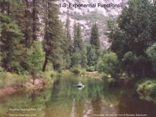
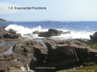
1.3 Exponential Functions Acadia National Park, Maine
Although some of today’s lecture is from the book, some of it is not. You must take notes to be successful in calculus.
The pictures in the lectures will usually illustrate the older TI-89. Although the buttons on the Titanium Edition are different shapes and colors, they are in the same positions and have the same functions. TI-89 We will be using the TI-89 calculator in this class. You may use either the TI-89 Titanium or the TI-84. TI-89 Titanium
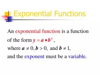
ENTER If $100 is invested for 4 years at 5.5% interest, compounded annually, the ending amount is: On the TI-89 TI 84 or N-Spire: At the end of each year, interest is paid on the amount in the account and added back into the account, so the amount of increase gets larger each year. This is an example of an exponential function: exponent base
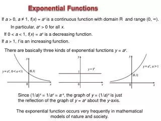
Where is ? Where is ? Where is ? Graph for in a [-5,5] by [-2,5] window:
Where is ? What is the domain? What is the range? Where is ? Where is ? Graph for in a [-5,5] by [-2,5] window:
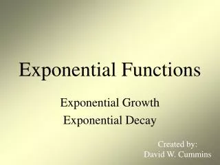
World Population: 1986 4936 million 1987 5023 1988 5111 1989 5201 1990 5329 1991 5422 Population growth can often be modeled with an exponential function: Ratio: The world population in any year is about 1.018 times the previous year. Nineteen years past 1991. in 2010: About 7.6 billion people.
Radioactive decay can also be modeled with an exponential function: Suppose you start with 5 grams of a radioactive substance that has a half-life of 20 days. When will there be only one gram left? After 20 days: 40 days: tdays: In Pre-Calc you solved this using logs. Today we are going to solve it graphically for practice.
WINDOW GRAPH Y=
WINDOW F5 GRAPH Upper bound and lower bound are x-values. 5 Intersection Math Use the arrow keys to select a first curve, second curve, lower bound and upper bound, and press ENTER each time. 46 days
Many real-life phenomena can be modeled by an exponential function with base , where . e can be approximated by: Graph: y=(1+1/x)^x in a [-10,10] by [-5,10] window. Use “trace” to investigate the function.
ENTER ENTER ENTER tbl………..1000 TblSet TABLE We can have the calculator construct a table to investigate how this function behaves as x gets much larger. tblStart …….1000 Move to the y1 column and scroll down to watch the y value approach e. p*
A regression equation starts with the points and finds the equation. The TI-89 has the exponential growth and decay model built in as an exponential regression equation.
To simplify, let represent 1880, represent 1890, etc. U.S. Population: 50.2 million 63.0 76.0 92.0 105.7 122.8 131.7 151.3 179.3 203.3 1880 1890 1900 1910 1920 1930 1940 1950 1960 1970 ENTER ENTER STO 0,1,2,3,4,5,6,7,8,9 2nd { 2nd } alpha L 1 (Upper case L used for clarity.) 6 3 2 alpha L 1 , alpha L 2 2nd MATH The calculator should return: ExpReg Done Statistics Regressions
ENTER ENTER 6 3 2 alpha L 1 , alpha L 2 2nd MATH The calculator should return: ExpReg Done Statistics Regressions 6 8 2nd MATH Statistics ShowStat The calculator gives you an equation and constants:
WINDOW ENTER ENTER Y= We can use the calculator to plot the new curve along with the original points: x y1=regeq(x) ) regeq 2nd VAR-LINK Plot 1
WINDOW GRAPH ENTER ENTER Plot 1
WINDOW GRAPH
F3 ENTER Trace What does this equation predict for the population in 1990? This lets us see values for the distinct points. This lets us trace along the line. 11 Enters an x-value of 11. Moves to the line.
ENTER What does this equation predict for the population in 1990? In 1990, the population was predicted to be 283.4 million. This is an over estimate of 33 million, or 13%. Why might this be? 11 Enters an x-value of 11.
To find the annual rate of growth: Since we used 10 year intervals with b=1.160626 : or p