Download
1 / 36
561 likes | 1.23k Vues
Chapter2. DISCRETE-TIME SIGNALS AND SYSTEMS. 2.0 Introduction 2.1 Discrete-Time Signals : Sequences 2.2 Discrete-Time Systems 2.3 Linear Time-Invariant Systems 2.4 Properties of Linear Time-Invariant Systems 2.5 Linear Constant-Coefficient Difference Equations

E N D
Chapter2. DISCRETE-TIME SIGNALS AND SYSTEMS 2.0 Introduction 2.1 Discrete-Time Signals : Sequences 2.2 Discrete-Time Systems 2.3 Linear Time-Invariant Systems 2.4 Properties of Linear Time-Invariant Systems 2.5 Linear Constant-Coefficient Difference Equations 2.6 Frequency-Domain Representation 2.7 Representation of Sequences of the Fourier Transform 2.8 Symmetry Properties of the Fourier Transform 2.9 Fourier Transform Theorems BGL/SNU
2.1.Discrete - Time Signals x[n]= x(t)|t=nT n : -1,0,1,2,… T: sampling period x(t) : analog signal ii) unit step sequence u[n] = 1, n0 0, n0 i) unit impulse signal(sequence) d[n] = 1, n=0 0, n0 BGL/SNU
iii) exponential/sinusoidal sequence x[n]= Aej(won+), Acos(won+) - not necessarily periodic in n with period 2p/wo - periodic in nwithperiod N (discrete number) for woN=2pk or wo= 2pk/N [note] x(t)= Ae j(wo t+) is periodic in t with period T= 2p/wo (continuous value) iv) general expression x[n] = Sx[k]d[n-k] BGL/SNU
x[n] y[n] T[ ] 2.2Discrete-Time Systems System : signal processor i) memoryless or with memory y[n] = f(x[n]), y[n]=f(x[n-k]) with delay ii) linearity x1[n]y1[n] x2[n]y2[n] a1x1[n] + a2x2[n] a1y1[n] + a2 y2[n] - e.g. T[a1x1[n] + a2x2[n]] = T[a1x1[n]] + T[a2x2[n]] = a1T[x1[n]] + a2T[x2[n]] BGL/SNU
iii) time-invariance x[n] y[n] x[n-n0] y[n-n0] - e.g., T[x[n-n0]] = T[x[n]] | n n-no - e.g., d[n] h[n] d[n-k] h[n-k] - counter-example : decimator T[ ] = x[Mn] iv) causality y[n] for n=n1, depends on x[n] for nn1 only - counter-example : y[n] = x[n+1] - x[n] BGL/SNU
v) stability bounded input yields bounded output(BIBO) |x[n]| < for all n |y[n]| < for all n - counter-example : y[n] = S u[k] = 0, n<0 n+1, n0 unbounded ( no fixed value By exists that keeps y[n] By < .) n k=- BGL/SNU
In general, let x[n] = Sx[k]d[n-k] In general, let x[n] = Sx[k]d[n-k] y[n] = T[ Sx[k]d[n-k]] k=- k 2.3 Linear Time-Invariant Systems d[n] h[n] LTI T[d[n]] : impulse response y[n] x[n] ( by linearity) = Sx[k]T[d[n-k]] k ( by time-invariance) = Sx[k]h[n-k] coefficient = x[n]*h[n] = Sx[n-r]h[r] r=- Convolution! BGL/SNU
d[n] = 1, n=0 0, n0 Sh[k]x[n-k] k=0 In summary, h[n] x[n] y[n] y[n] = x[n]*h[n] LTI h[n] : unique characteristic of the LTI system - causal LTI system y[n] = Sh[k]x[n-k] = k=- [note] h[n] = T[d[n]] = 0 n<0. as BGL/SNU
- Stable LTI System S | x[n-k] | • | h[k] | Sh[k]x[n-k] | |y[n]| = | k=- k=- S| h[k] | < By Bx k=- S| h[k] | Therefore, < k=- In fact, this is necessary and sufficient condition for stability of a BIBO system. ( You prove it! )(*1) BGL/SNU
~ ~ ~ x[n] y[n] y[n] - Example of non-LTI system - Decimator x[n] Decimator M y[n] = x[Mn] ? = x[n-1] = y[n-1] = x[M[n-1]] M=3 y[n] = x[Mn] BGL/SNU
~ y[n] y[n] y[n-1] No! = x[Mn-1] x[M[n-1]] = y[n-1] BGL/SNU
2.4 Properties of LTI System h[n] x[n] y[n] = x[n]*h[n] LTI i) parallel connection h[n] = h1[n] + h2[n] BGL/SNU
ii) cascade connection h[n] = h1[n]*h2[n] =h2[n]* h1[n] [note] distinctive feature of digital LTI system (*2) BGL/SNU
M M = Sbrx[n-r] = Sbrx[n-r] r = 0 r = 0 N Saky[n-k] k = 0 2.5 Linear Difference Equations LTI x[n] y[n] i) Case 1 : N=0 FIR System (set a0 =1, for convenience) y[n] For impulse input, x[n]=d[n], the response is h[n]= 0, n<0 or n>M br 0 n M finite impulse response! BGL/SNU
M = Sbrx[n-r] r = 0 N Saky[n-k] k = 1 ii) Case 2 : N 0 IIR System (set a0 =1, for convenience) y[n] e.g., set N=1 (lst order), and a1 = -a y[n] = b0 x[n] + ay[n-1] - For impulse input x[n] = d[n], the response is 1) If assume a causal system, i.e., y[n]=0 n<0. y[0] = b0 d[0] + ay[-1] = b0 y[1] = b0 d[1] + ay[0] = ab0 • • • y[n] = b0 d[n] + ay[n-1] = anb0 h[n] = anb0u[n] infinite impulse response! BGL/SNU
2) If assume an anti-causal system, i.e., y[n]=0 n>0. y[n-1] = a-1(-b0 d[n] + y[n]) y[0] = a-1(-b0 d[1] + y[1]) = 0 y[-1] = a-1(-b0 d[0] + y[0]) = a-1b0 h[n] = -anb0u[-n-1] • • • y[-n] = a-1(- b0 d[n+1] + y[n+1]) = -anb0 BGL/SNU
^ ^ y = Ax=lx y[n] = Sh[k] ejw(n-k) ^ ^ x x k = - 2.6 Frequency-Domain Representation • Linear System x y = Ax A scalar, eigenvalue for eigenvector input • LTI System x[n] y[n]=x[n]*h[n] h[n] y[n]=ejwn*h[n] ejwn = H(ejw)ejwn Fourier transform ( Sh[k] e-jwk )ejwn =H(ejw) ejwn = k = - BGL/SNU
Sh[k] e-jwk k = - p h[k] = 1/2p H(ejw) ejwkdw -p • Fourier Transform H(ejw) = You prove this! (*3) • Condition for existence of FT | X(ejw) | < S | x[n] | < “ absolutely summable” (BIBO stable condition) • Real - imaginary H(ejw) = HR(ejw) + j HI(ejw) BGL/SNU
• Magnitude-phase H(ejw) = | H(ejw) |ej H(ejw) (e.g.) ideal delay system x[n] y[n] = x[n-nd] h[n] y[n] = ejw(n-nd)= H(ejw) ejwn H(ejw) = e-jwnd ejwn HR(ejw) = coswnd HI(ejw) = - sinwnd | H(ejw) | = 1 H(ejw) = -wnd BGL/SNU
(e.g.) sinusoidal input x[n] = Acos(w0n + j) = (A/2) ejjejw0n + (A/2) e-jje-jw0n y[n] = H(ejw0) (A/2) ejjejw0n + H(e-jw0) (A/2) e-jje-jw0n = (A/2)(H(ejw0) ejjejw0n + H(e-jw0) e-jje-jw0n) y[n] = H(ejw) ejwn <1> = (A/2){ (H(ejw0) ejjejw0n ) + (H(ejw0) ejjejw0n)* } = ARe{H(ejw0) ejjejw0n} = A | H(ejw0) |(cosw0n + j + q) = A cos (w0(n-nd) + j) <2> <3> BGL/SNU
= ( Sh*[n] e-jw0n)* = H*(ejw0) n <1> if h[n] real h[n] = hR[n]+jhI[n] = hR[n] = h*[n] H(e-jw0) = Sh[n] e-(-jw0n) n <2> H(ejw) = | H(ejw) |ejq <3> if ideal delay system with | H(ejw) | = 1, H(ejw) = q = -wnd BGL/SNU
(e.g.) ideal lowpass filter (LPF) x[n] y[n] 1 -wc wc Hl(ejw) = 1. e-jwnd|w| 0. elsewhere wc periodic with period 2p Input x[n] = Acos(w0n + j) output y[n] = Acos(w0(n-nd )+ j) , if 0 , otherwise wo < wc BGL/SNU
sinw0[n-nd ] p[n-nd ] wc hl [k] = e-jwnd ejwndw -wc (e.g.) Fourier transform of anu[n] |a|<1 X(ejw) = Sane-jwn = S (ae-jw)n = n = 0 n = 0 (e.g.) inverse Fourier transform of ideal LPF = - <n < BGL/SNU
- Data length vs. Spectrum Change - Gibb’s phenomenon (page 52) BGL/SNU
- Error reduces in RMS sense but not in Chebyshev sense. Limitation of rectangular windowing BGL/SNU
2.8 Symmetry Properties (table 2.1) i) even / odd e : conjugate symmetric even o : conjugate anti-symmetric odd BGL/SNU
ii) real/imaginary iii) conjugation/reversal S = ( S )* BGL/SNU
iv) real/imaginary - even/odd v) for real x[n] real even imaginary odd BGL/SNU
(e.g.) x[n] = anu[n] |a|<1, real (example 2.25) even odd even odd BGL/SNU
2.9 Fourier Transform Theorems (table 2.2) i) linearity ii) time shifting iii) frequency shifting iv) time reversal BGL/SNU
v) differentiation in frequency vi) Parserval’s relation vii) convolution relation BGL/SNU
viii) modulation/windowing relation ix) fundamental functions BGL/SNU
1. 0. BGL/SNU
H.W. of Chapter 2 Matlab: [1] Consider the following discrete-time systems characterized by the difference equations: y[n]=0.5x[n]+0.27x[n-1]+0.77x[n-2] Write a MATLAB program to compute the output of the above systems for an input x[n]=cos(20n/256)+cos(200n/256), with 0n<299 and plot the output. [2] The Matlab command y=impz(num,den,N) can be used to compute the first N samples of the impulse response of the causal LTI discrete-time system. Compute the impulse response of the system described by y[n]-0.4y[n-1]+0.75y[n-2] =2.2403x[n]+2.4908x[n-1]+2.2403x[n-2] and plot the output using the stem function. BGL/SNU
H.W. of Chapter 2 Text: [3]2-15 [4]2-30 [5]2-42 [6]2-56 [7]2-58 BGL/SNU