Download
1 / 52
520 likes | 626 Vues
This is the second lecture concerning itself with the thermal modeling of buildings . This second example deals with the thermodynamic budget of Biosphere 2 , a research project located 50 km north of Tucson.

E N D
This is the second lecture concerning itself with the thermal modeling of buildings. This second example deals with the thermodynamic budget of Biosphere 2, a research project located 50 km north of Tucson. Since Biosphere 2 contains plant life, it is important, not only to consider the temperature inside the Biosphere 2 building, but also its humidity. The entire enclosure is treated like a single room with a single air temperature. The effects of air conditioning are neglected. The model considers the weather patterns at the location. Thermal Modeling of Buildings II
Biosphere 2: Original goals Biosphere 2: Revised goals Biosphere 2: Construction Biosphere 2: Biomes Conceptual model Bond graph model Conduction, convection, radiation Evaporation, condensation The Dymola model Simulation results Table of Contents
Biosphere 2 had been designed as a closed ecological system. The original aim was to investigate, whether it is possible to build a system that is materially closed, i.e., that exchanges only energy with the environment, but no mass. Such systems would be useful e.g. for extended space flights. Biosphere 2 contains a number of different biomes that communicate with each other. The model only considers a single biome. This biome, however, has the size of the entire structure. Air flow and air conditioning are being ignored. Biosphere 2: Original Goals
Later, Biosphere 2 was operated in a flow-through mode, i.e., the structure was no longer materially closed. Experiments included the analysis of the effects of varying levels of CO2 on plant grows for the purpose of simulating the effects of the changing composition of the Earth atmosphere on sustainability. Unfortunately, research at Biosphere 2 came to an almost still-stand around 2003 due to lack of funding. In 2007, management of Biosphere 2 was transferred to the University of Arizona. Hopefully, the change in management shall result in a revival of Biosphere 2 as an exciting experimental research facility for life sciences. Biosphere 2: Revised Goals
Biosphere 2 was built as a frame construction from a mesh of metal bars. The metal bars are filled with glass panels that are well insulated. During its closed operation, Biosphere 2 was slightly over-pressurized to prevent outside air from entering the structure. The air loss per unit volume was about 10% of that of the space shuttle! Biosphere 2: Construction I
The pyramidal structure hosts the jungle biome. The less tall structure to the left contains the pond, the marshes, the savannah, and at the lowest level, the desert. Though not visible on the photograph, there exists yet one more biome: the agricultural biome. Biosphere 2: Construction II
The two “lungs” are responsible for pressure equilibration within Biosphere 2. Each lung contains a heavy concrete ceiling that is flexibly suspended and insulated with a rubber membrane. If the temperature within Biosphere 2 rises, the inside pressure rises as well. Biosphere 2: Construction III Consequently, the ceiling rises until the inside and outside pressure values are again identical. The weight of the ceiling is responsible for providing a slight over-pressurization of Biosphere 2.
The (salt water) pond of Biosphere 2 hosts a fairly complex maritime ecosystem. Visible behind the pond are the marsh lands planted with mangroves. Artificial waves are being generated to keep the mangroves healthy. Above the cliffs to the right, there is the high savannah. Biosphere 2: Biomes I
This is the savannah. Each biome uses its own soil composition sometimes imported, such as in the case of the rain forest. Biosphere 2 has 1800 sensors to monitor the behavior of the system. Measurement values are recorded on average once every 15 Minutes. Biosphere 2: Biomes II
The agricultural biome can be subdivided into three separate units. The second lung is on the left in the background. Biosphere 2: Biomes III
The Biosphere 2 library is located at the top level of a high tower with a spiral staircase. Living in Biosphere 2 The view from the library windows over the Sonora desert is spectacular.
From the commando unit, it is possible to control the climate of each biome individually. For example, it is possible to program rain over the savannah to take place at 3 p.m. during 10 minutes. The Rain Maker
The climate control unit (located below ground) is highly impressive. Biosphere 2 is one of the most complex engineering systems ever built by mankind. Climate Control I
Beside from the temperature, also the humidity needs to be controlled. To this end, the air must be constantly dehumidified. The condensated water flows to the lowest point of the structure, located in one of the two lungs, where the water is being collected in a small lake; from there, it is pumped back up to where it is needed. Climate Control II
Temperature Humidity Condensation Evaporation The Bond-Graph Model • For evaporation, energy is needed. This energy is taken from the thermal domain. In the process, so-called latent heat is being generated. • In the process of condensation, the latent heat is converted back to sensible heat. • The effects of evaporation and condensation must not be neglected in the modeling of Biosphere 2.
These elements have been modeled in the manner presented earlier. Since climate control was not simulated, the convection occurring is not a forced convection, and therefore, it can essentially be treated like a conduction. Conduction, Convection, Radiation
Both evaporation and condensation can be modeled either as non-linear (modulated) resistors or as non-linear (modulated) transformers. Modeling them as transformers would seem a bit better, because they describe reversible phenomena. Yet in the model presented here, they were modeled as resistors. These phenomena were expressed in terms of equations rather than in graphical terms, since this turned out to be easier. Evaporation and Condensation
The overall Dymola model is shown to the left. At least, the picture shown is the top-level icon window of the model. The Dymola Model I
Night Sky Temperature Temperature of Dome Air Temperature Ambient Temperature Vegetation Temperature Air Humidity Soil Temperature Pond Temperature The Dymola Model II
Night Sky Radiation Solar Convection Solar Radiation Convection Evaporation and Condensation The Dymola Model III
e2 e1 Gth = G / T T T = e1+ e2 Convection Rth = R · T
e1 Gth = G · T 2 e1 T = e1 Radiation Rth = R / T 2
We first need to decide, which variables we wish to choose as effort and flow variables for describing humidity. A natural choice would have been to select the mass flow of evaporation as the flow variable, and the specific enthalpy of evaporation as the corresponding effort variable. Yet, this won’t work in our model, because we aren’t tracking any mass flows to start with. We don’t know, how much water is in the pond or how much water is stored in the leaves of the plants. We simply assume that there is always enough water, so that evaporation can take place, when conditions call for it. Evaporation and Condensation II
We chose the humidity ratio as the effort variable. It is measured in kg_water / kg_air. This is the only choice we can make. The units of flow must be determined from the fact that e·f = P. In this model, we did not use standard SI units. Time is here measured in h, and power is measured in kJ/h. Hence the flow variable must be measured in kJ·kg_air/(h·kg_water). Evaporation and Condensation III
The units of linear resistance follow from the resistance law: e = R·f. Thus, linear resistance is measured in h·kg_water2/(kJ·kg_air2). Similarly, the units of linear capacitance follow from the capacitive law: f = C·der(e). Hence linear capacitance is measured in kJ·kg_air2/kg_water2. R·C is a time constant measured in h. Evaporation and Condensation IV
Comparing with the literature, we find that our units for R and C are a bit off. In the literature, we find that Rhum is measured in h·kg_water/(kJ·kg_air), and Chum is measured in kJ·kg_air/kg_water. Hence the same non-linearity applies to the humidity domain that we had already encountered in the thermal domain: R = Rhum·e, and C = Chum/e. Evaporation and Condensation V
Thermal domain Humidity domain Programmed as equations Teten’s law } Sensible heat in = latent heat out Evaporation of the Pond
Programmed as equations If the temperature falls below the dew point, fog is created. Condensation in the Atmosphere
Ambient Temperature • In this example, the temperature values are stored as one long binary table. • The data are given in Fahrenheit. • Before they can be used, they must be converted to Kelvin.
Absorption, Reflection, Transmission Since the glass panels are pointing in all directions, it would be too hard to compute the physics of absorption, reflection, and transmission accurately, as we did in the last example. Instead, we simply divide the incoming radiation proportionally.
Distribution of Absorbed Radiation The absorbed radiation is railroaded to the different recipients within the overall Biosphere 2 structure.
The program works with weather data that record temperature, radiation, humidity, wind velocity, and cloud cover for an entire year. Without climate control, the inside temperature follows essentially outside temperature patterns. There is some additional heat accumulation inside the structure because of reduced convection and higher humidity values. Simulation Results I Air temperature inside Biosphere 2 without air-conditioning January 1 – December 31, 1995
Since water has a larger heat capacity than air, the daily variations in the pond temperature are smaller than in the air temperature. However, the overall (long-term) temperature patterns still follow those of the ambient temperature. Simulation Results II Water temperature inside Biosphere 2 without air-conditioning January 1 – December 31, 1995
The humidity is much higher during the summer months, since the saturation pressure is higher at higher temperature. Consequently, there is less condensation (fog) during the summer months. Indeed, it could be frequently observed during spring or fall evening hours that, after sun set, fog starts building up over the high savannah that then migrates to the rain forest, which eventually gets totally fogged in. Simulation Results III Air humidity inside Biosphere 2 without air-conditioning January 1 – December 31, 1995
Daily temperature variations in the summer months. The air temperature inside Biosphere 2 would vary by approximately 10oC over the duration of one day, if there were no climate control. Simulation Results IV Daily temperature variations during the summer months
Temperature variations during the winter months. Also in the winter, daily temperature variations would be close to 10oC. Simulation Results V • The humidity decreases as it gets colder. During day-time hours, it is higher than during the night.
The relative humidity is computed as the quotient of the true humidity and the humidity at saturation pressure. The atmosphere is almost always saturated. Only in the late morning hours, when the temperature rises rapidly, will the fog dissolve so that the sun may shine quickly. However, the relative humidity never decreases to a value below 94%. Only the climate control (not included in this model) makes life inside Biosphere 2 bearable. Simulation Results VI Relative humidity during three consecutive days in early winter.
In a closed system, such as Biosphere 2, evaporation necessarily leads to an increase in humidity. However, the humid air has no mechanism to ever dry up again except by means of cooling. Consequently, the system operates almost entirely in the vicinity of 100% relative humidity. The climate control is accounting for this. The air extracted from the dome is first cooled down to let the water fall out, and only thereafter, it is reheated to the desired temperature value. However, the climate control was not simulated here. Modeling of the climate control of Biosphere 2 is still being worked on. Simulation Results VII