Download

1 / 41
460 likes | 597 Vues
One-way Analysis of Variance. Limitations of the t-test. The t-test, although a useful tool, is limited to inferences regarding the differences between two means. If one wishes to use a t-test to analyze the differences between three means, one would have to conduct three separate t-tests.

E N D
Limitations of the t-test • The t-test, although a useful tool, is limited to inferences regarding the differences between two means. • If one wishes to use a t-test to analyze the differences between three means, one would have to conduct three separate t-tests. • For example, with three sample means (A, B, & C), one would have to find the difference between Mean A & Mean B, Mean A & Mean C, and Mean B & Mean C.
The Experiment-wise Type I Error Rate and the Bonferroni Correction • In addition to being tedious, this procedure would change the Type I error rate. • For example, if one conducted 20 t-tests, the probability of at least 1 one of these t-tests being significant at the α = .05 level of significance would be 5%. • In other words, with twenty t-tests, we would expect at least one test to be statistically significant because of chance alone. • The actual Type I error rate that should be used, in this instance, would be .05/20 = .0025. • This modified rate is called the Experiment-wise (or Family-wise) Type I error rate.
The Family-wise Type I Error Rate and the Bonferroni Correction • The statistic used to adjust for the family-wise Type I error rate is called the Bonferroni correction and is given by the formula: αFW = α J where J = number of tests and α = level of significance
Why Use ANOVA? • One problem with using such a small Type I error rate would be that the probability of making a Type II error would be greatly increased. • Furthermore, conducting multiple t-tests requires tedious calculation. • The ANOVA or Analysis of Variance is an answer to this problem.
When to Use ANOVA • It is feasible to use a one-way ANOVA when 1) the differences between two or more means is to be analyzed, 2) the dependent variable is a continuous variable, AND 3) the independent variable is a categorical variable. • Typically, the ANOVA is used whenever there are three or more means (although you can use it to analyze 2 means) • If more than one IV is used, a two-way (or higher) ANOVA is used. • If the same participants (or matched participants) are in all conditions, a repeated-measures ANOVA is used.
Historical Overview • The analysis of variance was created by Sir Ronald Aylmer Fisher, published in 1925 in his seminal textbook on statistics, “Statistical Methods for Research Workers”. • The original ANOVA that Fisher developed required converting the statistics into a specialized z (termed “Fisher’s z”) and required the statistician to use logarithms. • In 1934, George Snedecor greatly simplified this procedure, and derived the formula for the F-statistic commonly used today: F = MS Between / MS Within (note that Snedecor used statistical symbols in place of words). • Snedecor named the statistic as “F”, in honor of Ronald Fisher. • ANOVAs represent the most widely used statistical hypotheses tests performed in psychology today.
Assumptions of ANOVA • Assumptions of ANOVA: • The population is normally distributed. • Independence of observations. • Equal variances of comparison groups. • These are the same assumptions for the two sample t-test. • This is because the t-test is simply a special case of the ANOVA.
ANOVA and the t-test • The t-test analyzes the differences between the means. • The ANOVA analyzes the differences between the variances. • The mean is not squared. • The variance is squared. • The F statistic in the ANOVA analyzes the average sum of the squared differences between the means… • And the t-statistic in the t-test analyzes the differences between the means. • Hence, F = t²
The F-distribution • Another way to look at it is statistically: F = t² Therefore, all negative t values would become positive after squaring to become an F. Therefore, it is not possible to get a negative F value – in other words, only positive values of F are obtainable. The F-test only tests for the absolute differences between all of the groups (conditions) that are being compared. F of 0 = absolutely no difference between any of the conditions that are being compared.
The F-distribution • Another way to look at it is conceptually: The F-test compares the ratio of two differences (between- vs. within groups). • Null hypotheses for F tests are always non-directional because it is not possible to specify a direction of a difference when there is more than one direction involved • The values given in the F-distribution correspond to two-tailed values for the t-distribution.
The F-test As an illustration, refer to the t and F distribution tables: With 20 degrees of freedom, one-tailed, t=1.725 With 20 degrees of freedom, two-tailed, t=2.086 With 20 degrees of freedom in the denominator and 1 degree of freedom in the numerator (which corresponds to 20 degrees of freedom in the t-test), F=4.35 F=t² 2.086² = 4.35 but 1.725² = 2.98! The above is a mathematical illustration to show that values in the F-distribution are two-tailed t values
Significance in the ANOVA • When conducting a statistical test using the ANOVA, a ‘significant’ difference is found when the variance between the conditions exceeds the variance within the conditions by a statistically significant amount. • The variances, then, would include both sampling error and actual differences between the conditions. • This is because any differences due to sampling error would be accounted for by variance (or differences) within each of the conditions.
Significance in the ANOVA • Conceptually: • Significance = differences due to actual differences differences due to chance alone • As always, statistical significance depends upon the sample size and the Type I error rate (the alpha level or the level of significance). • However, the ANOVA only compares absolute differences between all three conditions (remember here that an analysis of variance contrasts the total variability between all groups). • In order to contrast the differences between specific means in an ANOVA, post-hoc tests are required.
Significance in the ANOVA • In statistical terms: • F = Mean Squares (MS) Between Mean Squares (MS) Within • In ANOVA, variance is denoted by the term ‘Mean Squares’ or MS for short. • The denominator reflects the standard error and the numerator reflects the treatment differences.
Significance in the ANOVA • Stated another way, significance in the ANOVA can also be conceptualized as: F = Variability due to the Effect Variability due to the Error
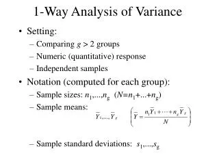
The One-way ANOVA table • J = number of conditions. • N = total number of participants, across all conditions (total sample size). • n = number of participants in a particular condition (sample size for a particular condition). • T = the sum of the scores in a particular condition. • X = an individual score.
The Mean Squares (MS) • The numerator of the sample variance formula represents the sum of squares (the sum of the squared differences from the mean). • In ANOVA, SSB represents the observed squared differences between conditions. • The denominator of the sample variance formula is the degrees of freedom. • Therefore,MS = Sample Variance
MS Between (MSB) • F = statistical significance. • Ceteris paribus, as MSB ↑, F ↑. • In other words, as the variability between the groups increases, the chances of finding a statistically significant effect increases. • As MSB ↑, power ↑. • In other words, as the variability between the groups increases, the ability of the hypothesis test to detect a statistically significant difference between the groups that are being compared increases. • In ANOVA, MSB = the systematic or explained variance. • To increase the variability between the groups, one could increase the strength of the experimental treatment. This will increase the discrepancy between the sample means
MS Between & Df Between • The denominator of the MSB formula is df Between. • Df Between = J – 1, where J = the number of conditions. • Ceteris paribus, as J ↑, MSB ↓. • As J ↑, power ↓. • In other words, as the number of conditions increases, the ability of the hypothesis test to detect a statistically significant difference between the groups that are being compared decreases.
MS Within (MSW) • Refer to the ANOVA table. • MS Within = SS Within / df Within. • Df Within = N –J • Contrast this with the standard error formula for the one-sample t-test : SM= S √ N • Notice that the structure of the statistic is the same for both formulas, whereby sample size appears on the denominator and sampling variability on the numerator
MS Within (MSW) • Hence, in ANOVA, MSW represents the standard error. • As MSW ↑, power ↓. • In other words, as standard error ↑, power ↓. • As SSW ↑, MSW ↑. • Error lowers statistical power. • Therefore, as SSW ↑, power ↓. • In other words, as standard deviation, which represents sample variability ↑, the ability of the hypothesis test to detect a statistically significant difference between the groups that are being compared decreases.
MSW & Df Within • Notice that df Within = N – J. • Therefore, as N ↑, df Within ↓. • Notice that MSW = SS Within /df Within • Therefore, as df Within ↑, MSW ↓ • Therefore, as N ↑, MSW ↓. • In other words, as sample size increases, the standard error decreases. • Because standard error is negatively related to statistical power, as N ↑, power ↑.
Statistical Significance • F is the bottom line, statistical significance. • F = MS Between MS Within • As MSB ↑, F ↑. • In other words, as the variability between conditions increases, power increases. • As MSW ↑, F ↓. • In other words, as the variability within conditions increases, power decreases.
Effect Size • Effect size in ANOVA is denoted by η² (eta squared). • In a one-way ANOVA, the variability due to the treatment is Sum of Squares Between, and the total variability is Sum of Squares Total. Hence, • η² = SS Between SS Total • Remember that d is just t free of sample size; similarly, eta-squared is just F free of sample size.
Example: One-way ANOVA Assume that an experiment with three conditions and a total of 15 participants has been conducted and that the results are as follows (assume that a six-point interval scale was used): Test the hypothesis at α=.05
Example: One-way ANOVA The first thing to calculate is Sum of Squares Total (SST). In order to do this, first calculate: ΣX² = 6² + 4² + 5² +3² + 3² + 5² + 3² + 3² + 4² + 2² + 0² + 1² + 1² + 4² + 2² = 36 + 16 + 25 + 9 + 9 + 25 + 9 +9 + 16 + 4 + 0 + 1 + 1 + 16 + 4 = 180
Example: One-way ANOVA Next, calculate (ΣX)² N = (6 + 4 + 5 + 3 + 3 + 5 + 3 + 3 + 4 + 2 + 0 + 1 + 1 + 4 + 2)² 15 (N = 15 in this experiment) = 46² = 2116 = 141.0715 15
Example: One-way ANOVA Therefore, SST = 180 – 141.07 = 38.93 Next, calculate Sum of Squares Between (SSB): Σ( T²) n = (6 + 4 + 5 + 3 + 3)² + (5 + 3 + 3 + 4 + 2 )² 5 5 + (0 + 1 + 1 + 4 + 2)² 5 = 441 + 289 + 64 = 88.2 + 57.8 + 12.8 = 158.8 5 5 5
Example: One-way ANOVA (ΣX)² was already calculated and was 141.07. N Therefore, SSB = Σ( T²) _ (ΣX)² n N = 158.8 – 141.07 = 17.73
Example: One-way ANOVA Next, calculate Sum of Squares Within (SSW) = SST – SSB = 38.93 – 17.73 = 21.2 Now, calculate all the degrees of freedom (df) df Between = J – 1 = 3 -1 = 2 df Within = N – J = 15 – 3 = 12 df Total = N – 1 = 15 – 1 = 14 As a check, notice that df Between + df Within = df Total
Example: One-way ANOVA Now, calculate Mean Squares Between (MSB) = SSB / df Between = 17.73 / 2 = 8.87 Now, calculate Mean Squares Within (MSW) = SSW / df Within = 21.2 / 12 = 1.77
Example: One-way ANOVA Finally, F = MSB MSW = 8.87 1.77 = 5.01This is the F-obtained.
Example: One-way ANOVA To look up the F-critical, you need to know three things: alpha level, df Between, and df Within For the F-table, df Between is read horizontally, and df Within is read vertically. At α=.05, df Between = 2, df Within = 12, F-critical = 3.88 Therefore, since 5.01 > 3.88, the results of this ANOVA are statistically significant at the .05 level of significance (reject Ho)
Example: One-way ANOVA • Calculate effect size • η² = SS Between/SS Total = 17.73/38.93 = .46
Write Up • The means and standard deviations are presented in Table 1. The analysis of variance indicated a significant difference, F(2, 12)= 5.01, p < .05, η2 = .46. Table 1. Means and Standard Deviations for each Condition
Post-hoc Tests • When you obtain a significant F-ratio, it simply indicates that somewhere among the entire set of mean differences there is at least one that is statistically significant. • Do NOT conduct post-hoc tests when ANOVA results are not significant! • Post-hoc tests are used after an ANOVA to determine exactly which mean differences are significant and which are not • We conduct pairwise comparisons, controlling for experiment-wise (or family-wise) alpha level • There are a variety of post-hoc tests that can be used
One Post-hoc test is Tukey’s HSD • Tukey’s HSD (honestly significant difference) • Determines the minimum difference between treatment means that is necessary for significance • If the mean difference between any two treatment conditions exceeds Tukey’s HSD, you conclude that there is a significant difference between those 2 treatments • HSD = q √(MSW/n) • Where q is found in table B.5 (p. 734) • MSW = within-treatements variance from the ANOVA • n = the number of scores in each treatment
In our example… • HSD = q √(MSW/n) = 3.77√(1.77/5) = 2.24 • Means: • Condition 1: 4.2 • Condition 2: 3.4 • Condition 3: 1.6 • Which means are different? • 4.2-3.4 = .8 • 3.4-1.6 = 1.8 • 4.2-1.6 = 2.6
Add to the write-up: • The means and standard deviations are presented in Table 1. The analysis of variance indicated a significant difference, F(2, 12)= 5.01, p < .05, η2 = .46. Post-hoc tests using Tukey’s HSD of 2.24 indicated that participants in condition 1 scored significantly higher (M = 4.2, SD = 1.30) than participants in condition 3 (M = 1.6, SD = 1.52). No other differences were found.