Download
1 / 12
120 likes | 197 Vues
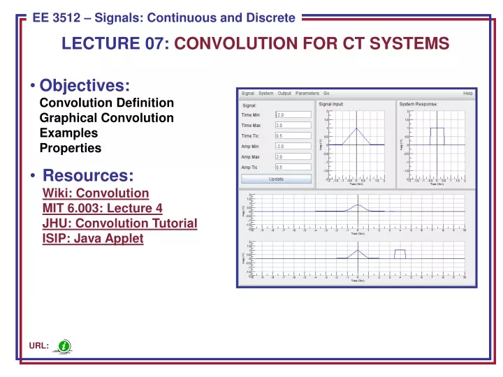
LECTURE 07: CONVOLUTION FOR CT SYSTEMS. Objectives: Convolution Definition Graphical Convolution Examples Properties Resources: Wiki: Convolution MIT 6.003: Lecture 4 JHU: Convolution Tutorial ISIP: Java Applet. URL:. Representation of CT Signals (Review).

E N D
LECTURE 07: CONVOLUTION FOR CT SYSTEMS • Objectives:Convolution DefinitionGraphical ConvolutionExamplesProperties • Resources:Wiki: ConvolutionMIT 6.003: Lecture 4JHU: Convolution TutorialISIP: Java Applet URL:
Representation of CT Signals (Review) • We approximate a CT signalas a weighted pulse function. • The signal can be written as a sum of these pulses: • In the limit, as : • Mathematical definition of an impulsefunction (the equivalent of the unit pulsefor DT signals and systems): • Unit pulses can be constructed from many functional shapes (e.g., triangular or Gaussian) as long as they have a vanishingly small width. The rectangular pulse is popular because it is easy to integrate
Response of a CT LTI System CT LTI • Denote the system impulse response, h(t), as the output produced when the input is a unit impulse function, (t). • From time-invariance: • From linearity: • This is referred to as the convolution integral for CT signals and systems. • Its computation is completely analogous to the DT version:
Example: Unit Pulse Functions • t < 0: y(t) = 0 • t > 2: y(t) = 0 • 0 t 1: y(t) = t • 1 t 2: y(t) = 2-t
Example: Negative Unit Pulse • t < 0.5: y(t) = 0 • t > 2.5: y(t) = 0 • 0.5 t 1.5: y(t) = 0.5-t • 1 t 2: y(t) = -2.5+t
Example: Combination Pulse • p(t) = 1 0 t 1 • x(t) = p(t) - p(t-1) • y(t) = ???
Example: Unit Ramp • p(t) = 1 0 t 1 • x(t) = r(t) p(t) • y(t) = ???
Properties of Convolution • Sifting Property: • Proof: • Integration: • Proof: • Step Response (follows from the integration property): • Comments: • Requires proof of the commutative property. • In practice, measuring the step response of a system is much easier than measuring the impulse response directly. How can we obtain the impulse response from the step response?
Properties of Convolution (Cont.) • Implications (from DT lecture): • Commutative Property: • Proof: • Distributive Property: • Proof:
Properties of Convolution (Cont.) • Implications (from DT lecture): • Associative Property: • Proof:
Useful Properties of CT LTI Systems • Causality: which implies: • This means y(t) only depends on x( < t). • Stability: Bounded Input ↔ Bounded Output Sufficient Condition: Necessary Condition:
Summary • We introduced CT convolution. • We worked some analytic examples. • We also demonstrated graphical convolution. • We discussed some general properties of convolution. • We also discussed constraints on the impulse response for bounded input / bounded output (stability).