Download

1 / 47
470 likes | 592 Vues
Learn about the divide-and-conquer paradigm, analysis, and implementation of Merge-sort and Quick-sort algorithms. Understand recursive calls, sorting sequences, and complexities.

E N D
Fall 2010 Data StructuresLecture 9 Fang Yu Department of Management Information Systems National Chengchi University
7 2 9 4 2 4 7 9 7 2 2 7 9 4 4 9 7 7 2 2 9 9 4 4 Fundamental Algorithms Divide and Conquer: Merge-sort, Quick-sort, and Recurrence Analysis
Divide-and-Conquer A general algorithm design paradigm Divide: divide the input data S in two or more disjoint subsets S1, S2, … Recur: solve the sub problems recursively Conquer: combine the solutions for S1,S2, …, into a solution for S The base case for the recursion are subproblems of constant size Analysis can be done using recurrence equations
Merge-sort • Merge-sort is a sorting algorithm based on the divide-and-conquer paradigm • Like heap-sort • It uses a comparator • It has O(n log n) running time • Unlike heap-sort • It does not use an auxiliary priority queue • It accesses data in a sequential manner (suitable to sort data on a disk)
Merge-sort • AlgorithmmergeSort(S, C) • Inputsequence S with n elements, comparator C • Outputsequence S sorted • according to C • ifS.size() > 1 • (S1, S2)partition(S, n/2) • mergeSort(S1, C) • mergeSort(S2, C) • Smerge(S1, S2) Merge-sort on an input sequence S with n elements consists of three steps: Divide: partition S into two sequences S1and S2 of about n/2 elements each Recur: recursively sort S1and S2 Conquer: merge S1and S2 into a unique sorted sequence
Merging Two Sorted Sequences • Algorithmmerge(A, B) • Inputsequences A and B withn/2 elements each • Outputsorted sequence of A B • S empty sequence • whileA.isEmpty() B.isEmpty() • ifA.first().element()<B.first().element() • S.addLast(A.remove(A.first())) • else • S.addLast(B.remove(B.first())) • whileA.isEmpty() S.addLast(A.remove(A.first())) • whileB.isEmpty() S.addLast(B.remove(B.first())) • return S The conquer step of merge-sort consists of merging two sorted sequences A and B into a sorted sequence S containing the union of the elements of A and B Merging two sorted sequences, each with n/2 elements and implemented by means of a doubly linked list, takes O(n) time
Merge-Sort Tree 7 2 9 4 2 4 7 9 7 2 2 7 9 4 4 9 7 7 2 2 9 9 4 4 • An execution of merge-sort is depicted by a binary tree • each node represents a recursive call of merge-sort and stores • unsorted sequence before the execution and its partition • sorted sequence at the end of the execution • the root is the initial call • the leaves are calls on subsequences of size 0 or 1
7 2 9 4 2 4 7 9 3 8 6 1 1 3 8 6 7 2 2 7 9 4 4 9 3 8 3 8 6 1 1 6 7 7 2 2 9 9 4 4 3 3 8 8 6 6 1 1 An execution example 7 2 9 4 3 8 6 11 2 3 4 6 7 8 9
7 2 2 7 9 4 4 9 3 8 3 8 6 1 1 6 7 7 2 2 9 9 4 4 3 3 8 8 6 6 1 1 Partition 7 2 9 4 3 8 6 11 2 3 4 6 7 8 9 7 2 9 4 2 4 7 9 3 8 6 1 1 3 8 6
7 7 2 2 9 9 4 4 3 3 8 8 6 6 1 1 Partition 7 2 9 4 3 8 6 11 2 3 4 6 7 8 9 7 2 9 4 2 4 7 9 3 8 6 1 1 3 8 6 7 2 2 7 9 4 4 9 3 8 3 8 6 1 1 6
7 2 2 7 9 4 4 9 3 8 3 8 6 1 1 6 Recur: base case 7 2 9 4 3 8 6 11 2 3 4 6 7 8 9 7 2 9 4 2 4 7 9 3 8 6 1 1 3 8 6 77 2 2 9 9 4 4 3 3 8 8 6 6 1 1
Recur: Base case 7 2 9 4 3 8 6 11 2 3 4 6 7 8 9 7 2 9 4 2 4 7 9 3 8 6 1 1 3 8 6 7 2 2 7 9 4 4 9 3 8 3 8 6 1 1 6 77 22 9 9 4 4 3 3 8 8 6 6 1 1
Merge 7 2 9 4 3 8 6 11 2 3 4 6 7 8 9 7 2 9 4 2 4 7 9 3 8 6 1 1 3 8 6 7 22 7 9 4 4 9 3 8 3 8 6 1 1 6 77 22 9 9 4 4 3 3 8 8 6 6 1 1
Recursive call,…, merge 7 2 9 4 3 8 6 11 2 3 4 6 7 8 9 7 2 9 4 2 4 7 9 3 8 6 1 1 3 8 6 7 22 7 9 4 4 9 3 8 3 8 6 1 1 6 77 22 9 9 4 4 3 3 8 8 6 6 1 1
Merge 7 2 9 4 3 8 6 11 2 3 4 6 7 8 9 7 2 9 42 4 7 9 3 8 6 1 1 3 8 6 7 22 7 9 4 4 9 3 8 3 8 6 1 1 6 77 22 9 9 4 4 3 3 8 8 6 6 1 1
Recursive call, …, merge, merge 7 2 9 4 3 8 6 11 2 3 4 6 7 8 9 7 2 9 42 4 7 9 3 8 6 1 1 3 6 8 7 22 7 9 4 4 9 3 8 3 8 6 1 1 6 77 22 9 9 4 4 33 88 66 11
Merge 7 2 9 4 3 8 6 11 2 3 4 6 7 8 9 7 2 9 42 4 7 9 3 8 6 1 1 3 6 8 7 22 7 9 4 4 9 3 8 3 8 6 1 1 6 77 22 9 9 4 4 33 88 66 11
Analysis of Merge-sort • The height h of the merge-sort tree is O(logn) • at each recursive call we divide in half the sequence, • The overall amount or work done at the nodes of depth iis O(n) • we partition and merge 2i sequences of size n/2i • we make 2i+1 recursive calls • Thus, the total running time of merge-sort is O(n log n)
Quick-sort x x L G E x A randomized sorting algorithm based on the divide-and-conquer paradigm: • Divide: pick a random element x (called pivot) and partition S into • L elements less than x • E elements equal x • G elements greater than x • Recur: sort L and G • Conquer: join L, Eand G
Partition Algorithmpartition(S,p) Inputsequence S, position p of pivot Outputsubsequences L,E, G of the elements of S less than, equal to, or greater than the pivot, resp. L,E, G empty sequences x S.remove(p) whileS.isEmpty() y S.remove(S.first()) ify<x L.addLast(y) else if y=x E.addLast(y) else{ y > x } G.addLast(y) return L,E, G • We partition an input sequence as follows: • We remove, in turn, each element y from S and • We insert y into L, Eor G,depending on the result of the comparison with the pivot x • Each insertion and removal is at the beginning or at the end of a sequence, and hence takes O(1) time • Thus, the partition step of quick-sort takes O(n) time
Quick-Sort Tree 7 4 9 6 2 2 4 6 7 9 4 2 2 4 7 9 7 9 2 2 9 9 • An execution of quick-sort is depicted by a binary tree • Each node represents a recursive call of quick-sort and stores • Unsorted sequence before the execution and its pivot • Sorted sequence at the end of the execution • The root is the initial call • The leaves are calls on subsequences of size 0 or 1
Execution Example 7 2 9 4 3 7 6 11 2 3 4 6 7 8 9 7 2 9 4 2 4 7 9 3 8 6 1 1 3 8 6 9 4 4 9 3 3 8 8 2 2 9 9 4 4 Pivot selection
Partition, recursive call, pivot selection 7 2 9 4 3 7 6 11 2 3 4 6 7 8 9 2 4 3 1 2 4 7 9 3 8 6 1 1 3 8 6 9 4 4 9 3 3 8 8 2 2 9 9 4 4 Quick-Sort
Partition, recursive call, base case 7 2 9 4 3 7 6 11 2 3 4 6 7 8 9 2 4 3 1 2 4 7 3 8 6 1 1 3 8 6 11 9 4 4 9 3 3 8 8 9 9 4 4 Quick-Sort
Recursive call, …, base case, join 7 2 9 4 3 7 6 11 2 3 4 6 7 8 9 2 4 3 1 1 2 3 4 3 8 6 1 1 3 8 6 11 4 334 3 3 8 8 9 9 44 Quick-Sort
Recursive call, pivot selection 7 2 9 4 3 7 6 11 2 3 4 6 7 8 9 2 4 3 1 1 2 3 4 7 9 7 1 1 3 8 6 11 4 334 8 8 9 9 9 9 44 Quick-Sort
Partition, …, recursive call, base case 7 2 9 4 3 7 6 11 2 3 4 6 7 8 9 2 4 3 1 1 2 3 4 7 9 7 1 1 3 8 6 11 4 334 8 8 99 9 9 44 Quick-Sort
Join, join 7 2 9 4 3 7 6 1 1 2 3 4 67 7 9 2 4 3 1 1 2 3 4 7 9 7 1779 11 4 334 8 8 99 9 9 44 Quick-Sort
In-place Quick-sort AlgorithminPlaceQuickSort(S,l,r) Inputsequence S, ranks l and r Output sequence S with the elements of rank between l and rrearranged in increasing order ifl r return i a random integer between l and r x S.elemAtRank(i) (h,k) inPlacePartition(x) inPlaceQuickSort(S,l,h - 1) inPlaceQuickSort(S,k + 1,r) • Quick-sort can be implemented to run in-place • In the partition step, we use replace operations to rearrange the elements • The recursive calls consider • elements with rank less than h • elements with rank greater than k
In-Place Quick-Sort j k (pivot = 6) 3 2 5 1 0 7 3 5 9 2 7 9 8 9 7 6 9 j k 3 2 5 1 0 7 3 5 9 2 7 9 8 9 7 6 9 • Perform the partition using two indices to split S into L, E, G • Repeat until j and k cross: • Scan j to the right until finding an element >x or j=k. • Scan k to the left until finding an element < x or j=k. • Swap elements at indices j and k (or swap pivot with j when j=k and return (j,j))
Recurrence Equation Analysis The conquer step of merge-sort consists of merging two sorted sequences, each with n/2 elements and implemented by means of a doubly linked list, takes at most bn steps, for some constant b. Likewise, the basis case (n< 2) will take at b most steps. Therefore, if we let T(n) denote the running time of merge-sort:
Recurrence Equation Analysis We can therefore analyze the running time of merge-sort by finding a closed form solution to the above equation. That is, a solution that has T(n) only on the left-hand side. We can achieve this by iterative substitution: In the iterative substitution, or “plug-and-chug,” technique, we iteratively apply the recurrence equation to itself and see if we can find a pattern
Iterative Substitution Note that base, T(n)=b, case occurs when 2i=n. That is, i = log n. So, Thus, T(n) is O(n log n).
The Recursion Tree Total time = bn + bn log n (last level plus all previous levels) Draw the recursion tree for the recurrence relation and look for a pattern:
Guess-and-Test Method In the guess-and-test method, we guess a closed form solution and then try to prove it is true by induction: For example: Guess: T(n) < cn log n
Guess-and-Test Method Wrong! We cannot make this last line be less than cn log n
Guess-and-Test Method, (cont.) So, T(n) is O(n log2n). In general, to use this method, you need to have a good guess and you need to be good at induction proofs. (if c>b) Recall the recurrence equation: Guess #2: T(n) < cn log2n.
Master Method Many divide-and-conquer recurrence equations have the form:
Master Method The Master Theorem:
Master Method, Example 1 • The form: • The Master Theorem: • Solution: • a = 4, b =2, f(n) is n • logba=2, so case 1 says T(n) is O(n2)
Master Method, Example 2 • The form: • The Master Theorem: • Solution: • a = 2, b =2 • Solution: logba=1, so case 2 says T(n) is O(n log2 n).
Master Method, Example 3 • The form: • The Master Theorem: • Solution: • a = 1, b =3 • logba=0, so case 3 says T(n) is O(n logn).
Master Method, Example 4 • The form: • The Master Theorem: • Solution: • a = 8, b =2 • logba=3, so case 1 says T(n) is O(n3).
HW9 (Due on Nov. 18) Quick sort keywords! Implement a quick sort algorithm for keywords Add each keyword into an array/linked list unorder Sort the keywords upon request Output all the keywords
Operations Given a sequence of operations in a txt file, parse the txt file and execute each operation accordingly
An input file Similar to HW7, add Fang 3 add Yu 5 add NCCU 2 add UCSB 1 output add MIS 4 Sort output You need to read the sequence of operations from a txt file 2. The format is firm 3. Raise an exception if the input does not match the format [Fang, 3][Yu, 5][NCCU, 2][UCSB, 1] [UCSB, 1][NCCU, 2][Fang, 3][MIS, 4] [Yu, 5]