Download
1 / 45
460 likes | 598 Vues
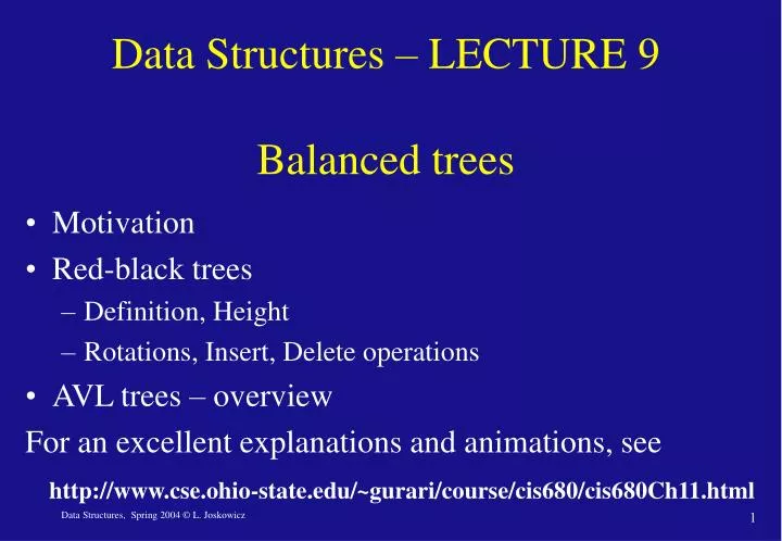
Data Structures – LECTURE 9 Balanced trees. Motivation Red-black trees Definition, Height Rotations, Insert, Delete operations AVL trees – overview For an excellent explanations and animations, see http://www.cse.ohio-state.edu/~gurari/course/cis680/cis680Ch11.html. Motivation.

E N D
Data Structures – LECTURE 9 Balanced trees • Motivation • Red-black trees • Definition, Height • Rotations, Insert, Delete operations • AVL trees – overview For an excellent explanations and animations, see http://www.cse.ohio-state.edu/~gurari/course/cis680/cis680Ch11.html
Motivation • Binary search trees are useful for efficiently implementing dynamic set operations: Search, Successor, Predecessor, Minimum, Maximum, Insert, Delete in O(h) time, where h is the height of the tree • When the tree is balanced, that is, its height h = O(lg n), the operations are indeed efficient. • However, the Insert and Delete alter the shape of the tree and can result in an unbalanced tree. In the worst case, h = O(n) no better than a linked list!
Balanced trees • We need to devise a method for keeping the tree balanced at all times. • When an Insert or Delete operation causes an imbalance, we want to correct this in at most O(lg n) time no complexity overhead. • To achieve this we need to augment the data structure with additional information and to devise tree-balancing operations. • The most popular balanced tree data structures: • Red-Black trees: height of at most 2(lg n + 1) • AVL trees: sub-tree height difference of at most 1.
Definition: Red-Black tree A red-black tree (RB tree) is a binary search tree where each node has an extra color bit (either red or black) with the following properties 1. Every node is either red or black. 2. The root is black. 3. Every leaf (null) is black. 4. Both children of a red node are black. 5. All paths from a node to its descendant leafs contain the same number of black nodes.
3 3 2 2 2 41 28 23 26 7 19 47 38 12 21 14 16 2 1 2 1 1 1 1 1 39 17 15 35 3 20 10 30 null null null null 1 1 1 1 1 null null 1 1 null null null null null black height next to nodes null null null null null null null null null null Example: Red-Black tree (1)
12 21 26 14 41 38 28 7 16 19 23 47 15 30 3 17 35 20 39 10 Example: Red-Black tree (2) null[T]
47 19 7 41 12 23 16 21 14 26 28 38 3 30 39 20 10 15 17 35 Example: Red-Black tree (3)
The height of Red-Black Trees (1) • Lemma: A red-black tree with n internal nodes has height at most 2 lg(n +1) • Definition: Black-height, bh(x), is the number of black nodes on any path from x to a leaf (not counting x itself). • Proof: We first prove a claim: The sub-tree rooted at any node x contains at least 2bh(x) –1 internal nodes. • We prove the claim by induction on the HEIGHT of the node h (not the black height.) • For h = 0, the node is a leaf. In this case bh(x) = 0. Then the claim implies that the number of internal nodes in the sub-tree rooted at the leaf is at least 20–1= 0, which is correct.
The height of Red-Black Trees (2) • For the induction step, consider x with h > 0, so x is an internal node and has two children, y and z. Then: • y is black bh(y) = bh(x)–1 • y is red bh(y) = bh(x) • Hence, bh(y) ≥bh(x)–1 • We can now use the induction assumption for y since its height (not black height!) is < than the height of x • Hence, the sub-tree rooted at y contains at least 2bh(x)–1 –1 internal nodes. • Multiplying this number by 2, for two sub-trees, and adding 1 for x, we get that the number of internal nodes in the sub-tree rooted by x is at least (2bh(x)–1 –1) + (2bh(x)–1 –1) + 1 = 2bh(x) –1
The height of Red-Black Trees (3) • Let h be the height of the tree and x be the root. We just proved that n≥ 2bh(x) –1 • By property 4, at least half of the nodes on any path from the root to a leaf (not including the root) must be black (cannot have two successive red nodes!) • Consequently, the black-height of the root is at least h/2 • Thus, the number of internal nodes n in the tree is n≥ 2h/2 –1 • We get: n +1≥ 2h/2 lg (n +1) ≥ 2 lg h/2 h≤2 lg (n+1)
Static operations in RB trees • The operations Max, Min, Search, Successor, and Predecessor take O(lg n) time in RB trees. • Proof: These operations can be applied exactly like in regular binary search trees, because they do not modify the tree, so the only difference is that the colors can be ignored. For binary search trees, we know that these operations take O(h) where h is the height of the tree, and by the lemma the height is O(lg n).
Dynamic operations in RB trees • The dynamic operations Insert and Delete change the shape of the tree. • Depending on the order of the operations, the tree can become unbalanced and loose the RB properties. • To maintain the RB structure, we must first change the colors some nodes in the tree and re-balance the tree by moving sub-trees around. • The re-balancing is done with the Rotation operation followed by a Re-coloring depending on the result.
Right-Rotate x Left-Rotate y α β δ Rotation operations (1) y x δ α β α ≤x ≤β and x ≤y ≤ δ α ≤x ≤y and β ≤y ≤ δ
Right-Rotate x y α β δ Rotation operations (2) y x δ Conflict: two Successive reds α β The rotation operation helps resolve the conflict!
Left-Rotate Left-Rotate(T,x)y right[x] /* Set y right[x] left[y] /* Turn y left’s sub-tree into x’s parent[left[y]] x /* right sub-tree parent[y] parent[x] /* Link x’s parent to y if parent[x] = null[T] then root[T] y else if x = left[parent[x]] thenleft[parent[x]] y else right[parent[x]] y left[y] x /* Put x on y’sleft parent[x] y
y 14 7 3 6 19 18 11 9 20 4 17 2 12 22 Example: Left-Rotate (1) x
y 14 7 3 6 19 18 11 α 22 9 20 17 2 12 4 β δ Example: Left-Rotate (2) x
14 7 3 6 18 11 19 α 17 4 2 20 12 22 9 β δ Example: Left-Rotate (3) y x
7 3 6 18 11 14 19 9 22 20 4 2 17 12 Example: Left-Rotate (4) y x
Rotation operations (2) • Preserves the properties of the binary search tree. • Takes constant time O(1) since it involves a constant number of pointer operations. • Left- and Right-Rotate are symmetric.
Red-Black Insert: principle (1) • Use ordinary binary search tree insertion and color the new node red. • If any of the red-black properties have been violated, fix the resulting tree using re-coloring and rotations. • Which of the five properties can be violated? • Every node is either red or black OK 2. The root is black. NO 3. Every null leaf is black OK 4. Both children of a red node are black NO 5. All paths from a node to its descendant leafs contain the same number of black nodes OK
Red-Black Insert: principle (2) • Violations: • 2. If the inserted x node is a root, paint it black OK • 4. What if the parent of the inserted node z is also red? • Three cases to fix this situations for node x: • Case 1: z’s uncle y is red • Case 2: z’s uncle y is black and z is a right child • Case 3: z’s uncle y is black and z is a left child
Recolor grandparent[z] new z C C parent[z] uncle[z] B D B D γ δ ε γ A A δ ε z α ß α ß Case 1: z’s uncle y is red • If z has both a red parent B and a red uncle D, re-color the parent and the uncle in black, and the grandparent C in red: • If C is the root, we can simply color it black. • If grandparent C is in violation, apply Cases 2 and 3.
Left-Rotate C C parent[z] uncle[z] A D D B α δ ε γ new z δ ε A B z γ ß α ß Case 2: z’s uncle y is black and z is a right child • If z is the right child of a red parent A and has a black uncle D, perform a left rotation A: • This produces a configuration handled by Case 3
Right-Rotate Re-color B grandparent[z] C A C parent[z] uncle[z] D γ z δ ε γ α ß D A α ß δ ε Case 3: z’s uncle y is black and z is a left child • If z is the left child of a red parent B and has a black uncle D, perform a right rotation at z’s grandparent C and re-color: B • After Case 3, there is no longer a violation!
RB-Insert • To insert a new node z into an RB-Tree, do: • Insert the new node z in the binary tree disregarding the colors. • Color z red • Fix the resulting tree if necessary by applying on z Cases 1, 2, and 3 as required and following their consequences • The complexity of the operation is O(lg n) • See Chapter 13 in textbook for code and proofs!
RB-Insert-Fixup (pseudo-code) RB-Insert-Fixup(T,z) whilecolor[parent[z]] = “red” doy z’s uncle ifcolor[y] = “red” thendo Case 1 else do ifz = right[parent[z]] thendo Case 2 do Case 3 color[root[T]] “black”
RB-Insert-Fixup loop invariants • Node z is red • If parent[z] is the root, then parent[z] is black • If there is a violation of the red-black properties, there is at most one violation and it is either of property 2 or 4. • If property 2 is violated, it is because z is root and red • If property 4 is violated, it is because both z and parent[z] are red.
11 1 7 14 parent[z] uncle[z] 2 5 8 15 4 inserted z Example: insertion and fixup (1) Violation: red node and red parent Case 1: z’s uncle is red re-color
uncle[z] 11 1 8 14 5 parent[z] 2 7 4 15 Example: insertion and fixup (2) z Violation: red node and red parent Case 2: z’s uncle is black and z is a right child left rotate
uncle[z] 11 1 8 14 5 parent[z] 7 2 4 15 Example: insertion and fixup (3) z Violation: red node and red parent Case 3: z’s uncle is black and z is a left child right rotate and re-color
7 1 5 14 8 2 15 4 11 Example: insertion and fixup (4) The tree has now RB properties No further fixing is necessary!
Red-Black Delete: principle (1) • Use ordinary binary search tree deletion. • If any of the red-black properties have been violated, fix the resulting tree using re-coloring and rotations. • Which of the five properties can be violated? • Every node is either red or black OK 2. The root is black. NO 3. Every null leaf is black OK 4. Both children of a red node are black NO 5. All paths from a node to its descendant leafs contain the same number of black nodes NO
Red-Black Delete: principle (2) • Violations: • If the parent y of the spliced node x is red, then properties 2, 4, 5 may be violated. • If x is red, re-coloring x black restores all of them! • So we are left with cases where both x and y are black. We need to restore property 5. • Four cases to fix this situation for node x: • Case 1: x’s sibling w is red • Case 2: x’s sibling w is black, as well as both children of w • Case 3: x’s sibling w is black, w’s left is red and right is black • Case 4: x’s sibling w is black, and w’s right child is red. y x
Left-Rotate Re-color D E B x x ε ζ w sibling[x] A C α ß γ α ß δ γ δ ε ζ Case 1: x’s sibling w is red • Case 1 is transformed into one of the Cases 2, 3, or 4 by switching the color of the nodes B and D and performing a left rotation: B w sibling[x] D A C E No change in black height!
Re-color new x D A α ß α ß C E x γ ζ γ δ ε δ ε ζ B B Case 2: x’s sibling w is black and both its children are black • Case 2 allows x to move one level up the tree by re-coloring D to “red”: w sibling[x] D A C E children[w] Decreases black height of nodes under D by one!
Right-Rotate Re-color B new w C A x x α ß α ß γ D γ δ ε δ ζ E ε ζ Case 3: x’s sibling w is black and its children are red and black • Case 3 is transformed to Case 4 by exchanging the colors of nodes C and D and performing a right rotation: B w sibling[x] D A C E children[w] No change in black height!
Left-Rotate Re-color D x E B α ß ε ζ A C γ δ ε ζ γ α ß δ Case 4: x’s sibling w is black and its right children is red • In this case, the violation is resolved by changing some colors and performing a left rotation without violating the red-black properties: B w sibling[x] D A C E children[w] Increases black height of nodes under A by one!
RB-Delete • To delete a node x from an RB-Tree, do: • Delete the node x fromthe binary tree disregarding the colors. • Fix the resulting tree if necessary by applying on x Cases 1, 2, 3, and 4 as required and following their consequences • The complexity of the operation is O(lg n) • See Chapter 13 in textbook for code and proofs!
RB-Delete-Fixup (pseudocode) RB-Delete-Fixup(T, x) whilex≠root[T] and color[x] = “black” do ifx = left[parent[x]] thenwx’s brother ifcolor[w] = “red” then do Case 1 // after this x stays, w changes to x’s new brother, and we are in Case 2 ifcolor[w] = “black” and its two children are black then do Case 2. // after this x moves to parent[x] else ifcolor[w] = “black” andcolor[right[w]] = “black” then do Case 3 // after this x stays, w changes to x’s new brother, and we are in Case 4 ifcolor[w] = “black” andcolor[right[w]] = “red” then do Case 4 // after this x = root[T]. else same as everything above but for x = right[parent[x]] color[x] “black”
RB-Delete: Complexity • If Case 2 is entered from Case 1, then we do not enter the loop again since x’s parent is red after Case 2. • If Case 3 or Case 4 are entered, then the loop is not entered again. • The only way to enter the loop many times is to enter through Case 2 and remain in Case 2. Hence, we enter the loop at most O(h) times. • This yields a complexity of O(lg n).
Summary of RB trees Important points to remember: • Five simple coloring properties guarantee a tree height of no more than 2(lg n + 1) = O(lg n) • Insertion and deletions are done as in uncolored binary search trees • Insertions and deletions can cause the properties of the RB tree to be violated. Fixing these properties is done by rotating and re-coloring parts of the tree • Violation cases must be examined individually. There are 3 cases for insertion and 4 or deletion. • In all cases, at most O(lg n) time is required.
x h Sh h-1 h-2 Sh-2 Sh-1 Sh=Sh–1 + Sh–2 AVL trees – definition Binary tree with a single balance property: For any node in the tree, the height difference between its left and right sub-trees is at most one.
AVL trees – properties • The height of an AVL tree is at most log1.3(n +1) h = O(lg n) • Keep an extra height field for every node • Four imbalance cases after insertion and deletion (instead of seven for RB trees) • See details in the Tirgul!
Summary • Efficient dynamic operations on a binary tree require a balance tree whose height is O(lg n) • There are various ways of guaranteeing a balanced height: • Red-black properties • Sub-tree height difference properties • B-trees properties • Insertion and deletion operations might require re-balancing in O(lg n) to restore balanced tree properties • Re-balancing operations require examining various cases