Download
1 / 61
610 likes | 795 Vues
Methods of Tree Reconstruction. Dan Graur. Molecular phylogenetic approaches: 1. distance-matrix (based on distance measures) 2. character-state (based on character states) 3. maximum likelihood (based on both character states and distances). DISTANCE-MATRIX METHODS

E N D
Methods of Tree Reconstruction Dan Graur
Molecular phylogenetic approaches: 1. distance-matrix (based on distance measures) 2. character-state (based on character states) 3. maximum likelihood (based on both character states and distances)
DISTANCE-MATRIX METHODS In the distance matrix methods, evolutionary distances (usually the number of nucleotide substitutions or amino-acid replacements between two taxonomic units) are computed for all pairs of taxa, and a phylogenetic tree is constructed by using an algorithm based on some functional relationships among the distance values.
Compute pairwise distances by correcting for multiple hits at a single sites Number of differences Number of changes (e.g., number of nucleotide substitutions, number of amino acid replacements)
Distance Matrix* *Units: Numbers of nucleotide substitutions per 1,000 nucleotide sites
Distance Methods: UPGMA Neighbor-relations Neighbor joining
UPGMA Unweighted pair-group method with arithmetic means
UPGMA employs a sequential clustering algorithm, in which local topological relationships are identified in order of decreased similarity, and the tree is built in a stepwise manner.
UPGMA yields the correct answer only if the distances are ultrametric! Q: What happens if the distances are only additive? Q: What happens if the distances are not even additive?
Neighborliness methods The neighbors-relation method(Sattath & Tversky) The neighbor-joining method (Saitou & Nei)
In an unrooted bifurcating tree, two OTUs are said to be neighbors if they are connected through a single internal node. Neighbors ≠ Sister Taxa
If we combine OTUs A and B into one composite OTU, then the composite OTU (AB) and the simple OTU C become neighbors.
A + + + C B D < = Four-Point Condition
In distance-matrix methods, it is assumed: Similarity Kinship
From Similarity to Relationship Similarities among OTUs can be due to: • Ancestry: • Shared ancestral characters (symplesiomorphies) • Shared derived characters (synapomorphy) • Homoplasy: • Convergent events • Parallel events • Reversals
Parsimony Methods: Willi Hennig 1913-1976
[Entities must not be multiplied beyond necessity] William of Occam (ca. 1285-1349) English philosopher & Franciscan monk William of Occam was “solemnly”excommunicated by Pope John XXII.
MAXIMUM PARSIMONY METHODS Maximum parsimony involves the identification of a topology that requires the smallest number of evolutionary changes to explain the observed differences among the OTUs under study. In maximum parsimony methods, we use discrete character states, and the shortest pathway leading to these character states is chosen as the “best” or maximum parsimony tree. Often two or more trees with the same minimum number of changes are found, so that no unique tree can be inferred. Such trees are said to be equally parsimonious.
In the case of four OTUs, an informative site can only favor one of the three possible alternative trees. Thus, the tree supported by the largest number of informative sites is the most parsimonious tree.
Inferring the maximum parsimony tree: 1. Identify all the informative sites. 2. For each possible tree, calculate the minimum number of substitutions at each informative site. 3. Sum up the number of changes over all the informative sites for each possible tree. 4. Choose the tree associated with the smallest number of changes as the maximum parsimony tree.
Maximum parsimony (Practice): • Data • TGCA • TACC • AGGT • AAGT • Step 1. Identify all the informative sites. ***
Maximum parsimony (Practice): • Data • TGC • TAC • AGG • AAG • Step 2. For each possible tree, calculate the minimum number of substitutions at each informative site.
Maximum parsimony (Practice): • Data • TGC • TAC • AGG • AAG • Step 3. Sum up the number of changes over all the informative sites for each possible tree. 4 5 6
Maximum parsimony (Practice): • Data • TGC • TAC • AGG • AAG • Step 4. Choose the tree associated with the smallest number of changes as the maximum parsimony tree. 4 5 6
Fitch’s (1971) method for inferring nucleotides at internal nodes The set at an internal node is the intersection () of the two sets at its immediate descendant nodes if the intersection is not empty. The set at an internal node is the union () of the two sets at its immediate descendant nodes if the intersection is empty. When a union is required to form a nodal set, a nucleotide substitution at this position must be assumed to have occurred.
4 substitutions 3 substitutions Fitch’s (1971) method for inferring nucleotides at internal nodes
Testing properties of ancestral proteins The ability to infer in silico the sequence of ancestral proteins, in conjunction with some astounding developments in synthetic biology, allow us to “resurrect” putative ancestral proteins in the laboratory and test their properties. These properties, in turn, can be used to test hypotheses concerning the physical environment which the ancestral organism inhabited (its paleoenvironment).
Testing properties of ancestral proteins Gaucher et al. (2003) used EF-Tu (Elongation-Factor thermounstable) gene sequences from completely sequenced mesophile eubacteria to reconstruct candidate ancestral sequences at nodes throughout the bacterial tree. These inferred ancestral proteins were, then, synthesized in the laboratory, and their activities and thermal stabilities were measured and compared to those of extant organisms. Thermostability curves The temperature profile of the inferred ancestral protein was 55°C, suggesting that the ancestor of extant mesophiles was a thermophile.
Ancestral reconstruction is not possible with morphological data.
The impossibility of exhaustively searching for the maximum-parsimony tree when the number of OTUs is large