Download
1 / 52
520 likes | 649 Vues
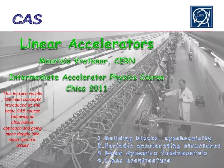
Linear Accelerators Maurizio Vretenar, CERN Intermediate Accelerator Physics Course Chios 2011. This lecture recalls the main concepts introduced at the basic CAS course following an alternative approach and going more deeply into some specific issues . Building blocks, synchronicity

E N D
Linear Accelerators Maurizio Vretenar, CERNIntermediate Accelerator Physics Course Chios 2011 This lecture recalls the main concepts introduced at the basic CAS course following an alternative approach and going more deeply into some specific issues • Building blocks, synchronicity • Periodic accelerating structures • Beam dynamics fundamentals • Linac architecture
Why Linear Accelerators Linear Accelerators are used for: Low-Energy accelerationof protons and ions (injectors to synchrotrons or stand-alone): linacs can be synchronous with the RF fields in the range where velocity increases with energy. When velocity is ~constant, synchrotrons are more efficient (multiple crossings of the RF gaps instead of single crossing). Protons : b = v/c =0.51 at 150 MeV, 0.95 at 2 GeV. High-Energy accelerationof high-intensity proton beams: in comparison with synchrotrons,linacs can go to higher repetition rate, are less affected by resonances and have more distributed beam losses.Higher injection energy from linacs to synchrotrons leads to lower space charge effects in the synchrotron and allows increasing the beam intensity. Low and High-Energy accelerationof electron beams : in linacs electrons don’t lose energy because of synchrotron radiation. Electron linacs are simple and compact (more than 5’000 e-linacs in the world for cancer therapy!), can be used for many applications (as the FEL) and are the only option to reach very high energies (ILC and CLIC). 3
Definitions In linear accelerators the beam crosses only once the accelerating structures. Protons, ions: used in the region where the velocity of the particle beam increases with energy Electrons: used at all energies. The periodicity of the RF structure must match the particle velocity → development of a complete panoply of structures (NC and SC) with different features. Protons and ions: at the beginning of the acceleration, beta (=v/c) is rapidly increasing, but after few hundred MeV’s (protons) relativity prevails over classical mechanics (b~1) and particle velocity tends to saturate at the speed of light. The region of increasing b is the region of linear accelerators. The region of nearly constant bis the region of synchrotrons. Electrons: Velocity=c above few keV (protons, classical mechanics) (v/c)2 electrons protons W
Basic linear accelerator structure RF cavity Focusing magnet B-field DC particle injector bunching section E-field ? d Protons: energy ~100 keV b= v/c ~ 0.015 Accelerating gap: E = E0 cos (wt + f) en. gain DW = eV0Tcosf Acceleration the beam has to pass in each cavity on a phase f near the crest of the wave The beam must to be bunched at frequency w distance between cavities and phase of each cavity must be correlated Phase change from cavity i to i+1 is For the beam to be synchronous with the RF wave (“ride on the crest”) phase must be related to distance by the relation: … and on top of acceleration, we need to introduce in our “linac” some focusing elements 5 … and on top of that, we will couple a number of gaps in an “accelerating structure”
Accelerating structure architecture When b increases during acceleration, either the phase difference between cavities Dfmust decrease or their distance d must increase. d = const. f variable d Individual cavities – distance between cavities constant, each cavity fed by an individual RF source, phase of each cavity adjusted to keep synchronism, used for linacs required to operate with different ions or at different energies. Flexible but expensive! Better, but 2 problems: create a “coupling”; create a mechanical and RF structure with increasing cell length. f = const. d variable d bl Coupled cell cavities - a single RF source feeds a large number of cells (up to ~100!) - the phase between adjacent cells is defined by the coupling and the distance between cells increases to keep synchronism . Once the geometry is defined, it can accelerate only one type of ion for a given energy range. Effective but not flexible.
Case 1: a single-cavity linac The goal is flexibility: acceleration of different ions (e/m) at different energies need to change phase relation for each ion-energy RF cavity focusing solenoid REX-HIE linac (to be built at CERN - superconducting) Post-accelerator of radioactive ions 2 sections of identical equally spaced cavities Quarter-wave RF cavities, 2 gaps 12 + 20 cavities with individual RF amplifiers, 8 focusing solenoids Energy 1.2 10 MeV/u, accelerates different A/m beam 7
Case 2 : a Drift Tube Linac d 10 MeV, b = 0.145 50 MeV, b = 0.31 Tank 2 and 3 of the new Linac4 at CERN: 57 coupled accelerating gaps Frequency 352.2 MHz, l = 85 cm Cell length (d=bl) from 12.3 cm to 26.4 cm (factor 2 !). 8
Intermediate cases • But: • Between these 2 “extremes” there are many “intermediate” cases, because: • Single-gap cavities are expensive (both cavity and RF source!). • Structures with each cell matched to the beta profile are mechanically complicated and expensive. • → as soon as the increase of beta with energy becomes small (Db/DW) we can accept a small error and: • Use multi-gap cavities with constant distance between gaps. • Use series of identical cavities (standardised design and construction). 9 9
Synchronism condition in a multi-cell cavity The distance between accelerating gaps is proportional to particle velocity Example: a linac superconducting 4-cell accelerating structure Synchronism condition bw. particle and wave t (travel between centers of cells) = T/2 d=distance between centres of consecutive cells “phase slippage” In an ion linac cell length has to increase (up to a factor 200 !), the linac will be made of a sequence of different accelerating structures (changing cell length, frequency, operating mode, etc.) matched to the ion velocity. In sequences of (few) identical cells where b increases (acceleration) only the central cell will be synchronous, and in the other cells the beam will have a phase error. = phase error on a gap for a particle with b+Db crossing a cell designed for b High and unacceptable for low energy, becomes lower and acceptable for high b
Sections of identical cavities: a superconducting linac (medium b) The same superconducting cavity design can be used for different proton velocities. The linac has different sections, each made of cavities with cell length matched to the average beta in that section. At “medium energy” (>150 MeV) we are not obliged to dimension every cell or every cavity for the particular particle beta at that position, and we can accept a slight “asynchronicity” → phase slippage + reduction in acceleration efficiency from the optimum one. b=0.52 b=0.7 b=0.8 b=1 11 CERN (old) SPL design, SC linac 120 - 2200 MeV, 680 m length, 230 cavities
Multi-gap coupled-cell cavities Between these 2 extreme case (array of independently phased single-gap cavities / single long chain of coupled cells with lengths matching the particle beta) there can be a large number of variations (number of gaps per cavity, length of the cavity, type of coupling) each optimized for a certain range of energy and type of particle. The goal of this lecture is to provide the background to understand the main features of these different structures… DTL SCL CH PIMS CCDTL 12
Linear and circular accelerators accelerating gaps d accelerating gap d d=bl/2=variable d=2pR=constant Linear accelerator: Particles accelerated by a sequence of gaps (all at the same RF phase). Distance between gaps increases proportionally to the particle velocity, to keep synchronicity. Used in the range where b increases. “Newton” machine Circular accelerator: Particles accelerated by one (or more) gaps at given positions in the ring. Distance between gaps is fixed. Synchronicity only for b~const, or varying (in a limited range!) the RF frequency. Used in the range where b is nearly constant. “Einstein” machine 13
Electron linacs In an electron linac velocity is ~ constant. For using the fundamental accelerating mode cell length must be d = bl / 2. the linac structure will be made of a sequence of identical cells. Because of the limits of the RF source, the cells will be grouped in cavities operating in travelling wave mode. 14 Pictures from K. Wille, The Physics of Particle Accelerators
(Proton) linac building blocks HV AC/DC power converter AC to DC conversion efficiency ~90% Main oscillator DC to RF conversion efficiency ~50% RF feedback system High power RF amplifier (tube or klystron) RF to beam voltage conversion efficiency = SHUNT IMPEDANCE ZT2 ~ 20 - 60 MW/m DC particle injector buncher ion beam, energy W magnet powering system vacuum system water cooling system LINAC STRUCTURE accelerating gaps + focusing magnets designed for a given ion, energy range, energy gain 15
Conclusions – part 1 • What did we learn? • A linac is composed of an array of accelerating gaps, interlaced with focusing magnets (quadrupoles or solenoids), following an ion source with a DC extraction and a bunching section. • When beam velocity is increasing with energy (“Newton” regime), we have to match to the velocity (or to the relativistic b) either the phase difference or the distance between two subsequent gaps. • We have to compromise between synchronicity (distance between gaps matched to the increasing particle velocity) and simplicity (number of gaps on the same RF source, sequences of identical cavities). At low energies we have to follow closely the synchronicity law, whereas at high energies we have a certain freedom in the number of identical cells/identical cavities. • Proton and electron linacs have similar architectures; proton linacs usually operate in standing wave mode, and electron linacs in traveling wave mode. 17
Coupling accelerating cells 1. Magnetic coupling: open “slots” in regions of high magnetic field B-field can couple from one cell to the next 2. Electric coupling: enlarge the beam aperture E-field can couple from one cell to the next How can we couple together a chain of n accelerating cavities ? The effect of the coupling is that the cells no longer resonate independently, but will have common resonances with well defined field patterns. 19
A 7-cell magnetically-coupled structure: the PIMS PIMS = Pi-Mode Structure, will be used in Linac4 at CERN to accelerate protons from 100 to 160 MeV RF input This structure is composed of 7 accelerating cells, magnetically coupled. The cells in a cavity have the same length, but they are longer from one cavity to the next, to follow the increase in beam velocity. 20
Linac cavities as chains of coupled resonators What is the relative phase and amplitude between cells in a chain of coupled cavities? R A linear chain of accelerating cells can be represented as a chain of resonant circuits magnetically coupled. Individual cavity resonating at w0 frequenci(es) of the coupled system ? Resonant circuit equation for circuit i (R0): M M L L L Ii L C Dividing both terms by 2jwL: General response term, (stored energy)1/2, can be voltage, E-field, B-field, etc. Contribution from adjacent oscillators General resonance term 21
The Coupled-system Matrix A chain of N+1 resonators is described by a (N+1)x(N+1) matrix: or This matrix equation has solutions only if • Eigenvalue problem! • System of order (N+1) in w only N+1 frequencies will be solution of the problem (“eigenvalues”, corresponding to the resonances) a system of N coupled oscillators has N resonance frequencies an individual resonance opens up into a band of frequencies. • At each frequency wi will correspond a set of relative amplitudes in the different cells (X0, X2, …, XN): the “eigenmodes” or “modes”. 22
Modes in a linear chain of oscillators We can find an analytical expression for eigenvalues (frequencies) and eigenvectors (modes): the index q defines the number of the solution is the “mode index” Frequencies of the coupled system : • Each mode is characterized by a phase pq/N. Frequency vs. phase of each mode can be plotted as a “dispersion curve” w=f(f): • each mode is a point on a sinusoidal curve. • modes are equally spaced in phase. w0/√1-k w0 w0/√1+k p 0 p/2 The “eigenvectors = relative amplitude of the field in the cells are: STANDING WAVE MODES, defined by a phase pq/N corresponding to the phase shift between an oscillator and the next one pq/N=F is the phase difference between adjacent cells that we have introduces in the 1st part of the lecture. 23
Example: Acceleration on the normal modes of a 7-cell structure 0 w = w0/√1+k 0 (or 2p) mode, acceleration if d = bl Intermediate modes p/2 w = w0 p/2 mode, acceleration if d = bl/4 … w = w0/√1-k p 24 p mode, acceleration if d = bl/2, Note: Field always maximum in first and last cell!
Practical linac accelerating structures Note: our relations depend only on the cell frequency w, not on the cell length d !!! As soon as we keep the frequency of each cell constant, we can change the cell length following any acceleration (b) profile! Example: The Drift Tube Linac (DTL) Chain of many (up to 100!) accelerating cells operating in the 0 mode. The ultimate coupling slot: no wall between the cells! Each cell has a different length, but the cell frequency remains constant “the EM fields don’t see that the cell length is changing!” d (L , C↓) LC ~ const w ~ const 25
The DTL Standing wave linac structure for protons and ions, b=0.1-0.5, f=20-400 MHz Drift tubes are suspended by stems (no net RF current on stem) Coupling between cells is maximum (no slot, fully open !) The 0-mode allows a long enough cell (d=bl) to house focusing quadrupoles inside the drift tubes! E-field B-field 26
Examples of DTL Top; CERN Linac2 Drift Tube Linac accelerating tank 1 (200 MHz). The tank is 7m long (diameter 1m) and provides an energy gain of 10 MeV. Left: DTL prototype for CERN Linac4 (352 MHz). Focusing is provided by (small) quadrupoles inside drift tubes. Length of drift tubes (cell length) increases with proton velocity. 27
The Linac4 DTL 352 MHz frequency Tank diameter 500mm 3 resonators (tanks) Length 19 m 120 Drift Tubes Energy 3 MeV to 50 MeV Beta 0.08 to 0.31 cell length (bl) 68mm to 264mm factor 3.9 increase in cell length beam 28
Multi-gap Superconducting linac structures (elliptical) Standing wave structures for particles at b>0.5-0.7, widely used for protons (SNS, etc.) and electrons (ILC, etc.) f=350-700 MHz (protons), f=350 MHz – 3 GHz (electrons) Chain of cells electrically coupled, large apertures (ZT2 not a concern). Operating in p-mode, cell length bl/2 Input coupler placed at one end. 29
The normal conducting zoo For normal-conducting, the goal is designing high-efficiency structures with a large number of cells (higher power RF sources are less expensive). Two important trends: Use p/2 modes for stability of long chains of resonators → CCDTL (Cell-Coupled Drift Tube Linac), SCL (Side Coupled Linac), ACS (Annular Coupled Structure),.... Use alternative modes: H-mode structures (TE band) → Interdigital IH, CH DTL SCL CH 30 30 PIMS CCDTL
The superconducting zoo Spoke (low beta) [FZJ, Orsay] QWR (low beta) [LNL, etc.] CH (low/medium beta) [IAP-FU] 10 gaps 2 gaps Re-entrant [LNL] 4 gaps HWR (low beta) [FZJ, LNL, Orsay] 4 to 7 gaps 2 gaps 1 gap Superconducting structure for linacs can have a small number of gaps → used for low and medium beta. Elliptical structures with more gaps (4 to 7) are used for medium and high beta. Elliptical cavities [CEA, INFN-MI, CERN, …] 31
Traveling wave accelerating structures (electrons) What happens if we have an infinite chain of oscillators? becomes (Nh) becomes (Nh) All modes in the dispersion curve are allowed, the original frequency degenerates into a continuous band. The field is the same in each cell, there are no more standing wave modes only “traveling wave modes”, if we excite the EM field at one end of the structure it will propagate towards the other end. w0/√1-k w0 w0/√1+k 0 p/2 p But: our dispersion curve remains valid, and defines the velocity of propagation of the travelling wave, vf = wd/F For acceleration, the wave must propagate at vf= c for each frequency w and cell length d we can find a phase F where the apparent velocity of the wave vf is equal to c 32
Traveling wave accelerating structures How to “simulate” an infinite chain of resonators? Instead of a singe input, exciting a standing wave mode, use an input + an output for the RF wave at both ends of the structure. beam “Disc-loaded waveguide” or chain of electrically coupled cells characterized by a continuous band of frequencies. In the chain is excited a “traveling wave mode” that has a propagation velocity vph = w/k given by the dispersion relation. For a given frequency w, vph = c and the structure can be used for particles traveling at b=1 The “traveling wave” structure is the standard linac for electrons from b~1. • Can not be used for protons at v<c: 1. constant cell length does not allow synchronism 2. structures are long, without space for transverse focusing 33
Examples: a TW accelerating structure A 3 GHz LIL accelerating structure used for CTF3. It is 4.5 meters long and provides an energy gain of 45 MeV. One can see 3 quadrupoles around the RF structure. 34
Examples: an electron linac RF input RF output Focusing solenoids Accelerating structure (TW) The old CERN LIL (LEP Injector Linac) accelerating structures (3 GHz). The TW structure is surrounded by focusing solenoids, required for the positrons. 35
Conclusions – part 2 • What did we learn? • Coupling together accelerating cells (via the magnetic or electric field) is a way to fix their phase relation. • A chain of N coupled resonators will always have N modes of oscillation. Each mode will have a resonance frequency and a field pattern with a corresponding phase shift from cell to cell. • Choosing the excitation frequency, we can decide in which mode to operate the structure, and we can select a mode with a phase advance between cells suitable for acceleration. If we change the length of a cell without changing its frequency, we can follow the increase the particle velocity. • Practical linac structures operate either on mode 0 (DTL), less efficient but leaving space for internal focusing elements, or on mode p, standard for multi-cell cavities. More exotic modes (p/2, TE) are used in special cases. • Electron linacs operate with long chains of identical cells excited by a traveling wave, propagating at the (constant) velocity of the beam. 36
Longitudinal dynamics • Ions are accelerated around a (negative = linac definition) synchronous phase. • Particles around the synchronous one perform oscillations in the longitudinal phase space. • Frequency of small oscillations: • Tends to zero for relativistic particles g>>1. • Note phase damping of oscillations: At relativistic velocities phase oscillations stop, and the beam is compressed in phase around the initial phase. The crest of the wave can be used for acceleration. 38
Longitudinal dynamics - electrons • Electrons at v=c remain at the injection phase. • Electrons at v<c injected into a TW structure designed for v=c will move from injection phase j0 to an asymptotic phase j, which depends only on gradient and b0 at injection. • The beam can be injected with an offset in phase, to reach the crest of the wave at b=1 • Capture condition, relating E0 and b0 : Example: l=10cm, Win=150 keV and E0=8 MV/m. In high current linacs, a bunching and pre-acceleration sections up to 4-10 MeV prepares the injection in the TW structure (that occurs already on the crest) 39
Transverse dynamics - Space charge • Large numbers of particles per bunch ( ~1010 ). • Coulomb repulsion between particles (space charge) plays an important role. • But space charge forces ~ 1/g2 disappear at relativistic velocity Force on a particle inside a long bunch with density n(r) traveling at velocity v: B E 40
Transverse dynamics - RF defocusing • RF defocusing experienced by particles crossing a gap on a longitudinally stable phase. • In the rest frame of the particle, only electrostatic forces no stable points (maximum or minimum) radial defocusing. • Lorentz transformation and calculation of radial momentum impulse per period (from electric and magnetic field contribution in the laboratory frame): Bunch position at max E(t) • Transverse defocusing~ 1/g2 disappears at relativistic velocity (transverse magnetic force cancels the transverse RF electric force). 41
Transverse beam equilibrium in linacs The equilibrium between external focusing force and internal defocusing forces defines the frequency of beam oscillations. Oscillations are characterized in terms of phase advance per focusing periodstor phase advance per unit lengthkt. Ph. advance = Ext. quad focusing - RF defocusing - space charge q=charge G=quad gradient l=length foc. element f=bunch form factor r0=bunch radius l=wavelength … Approximate expression valid for: F0D0 lattice, smooth focusing approximation, space charge of a uniform 3D ellipsoidal bunch. A “low-energy” linac is dominated by space charge and RF defocusing forces !! Phase advance per period must stay in reasonable limits (30-80 deg), phase advance per unit length must be continuous (smooth variations) at low b, we need a strong focusing term to compensate for the defocusing, but the limited space limits the achievable G and l needs to use short focusing periods N bl. Note that the RF defocusing term f sets a higher limit to the basic linac frequency (whereas for shunt impedance considerations we should aim to the highest possible frequency, Z √f). 42 42
Focusing periods Focusing usually provided by quadrupoles. Need to keep the phase advance in the good range, with an approximately constant phase advance per unit length → The length of the focusing periods has to change along the linac, going gradually from short periods in the initial part (to compensate for high space charge and RF defocusing) to longer periods at high energy. For Protons(high beam current and high space charge), distance between two quadrupoles (=1/2 of a FODO focusing period): - blin the DTL, from ~70mm (3 MeV, 352 MHz) to ~250mm (40 MeV), - can be increased to 4-10bl at higher energy (>40 MeV). - longer focusing periods require special dynamics (example: the IH linac). For Electrons (no space charge, no RF defocusing): focusing periods up to several meters, depending on the required beam conditions. Focusing is mainly required to control the emittance. 43
Conclusions – part 3 • What did we learn? • Transverse beam dynamics in linacs is dominated by space charge and RF defocusing forces. • In order to keep the transverse phase advance within reasonable limits, focusing has to be strong (large focusing gradients, short focusing periods) at low energy, and can then be relaxed at higher energy. • A usual linac is made of a sequence of structures, matched to the beam velocity, and where the length of the focusing period increases with energy. • The very low energy section remains a special problem next lecture 44
Architecture: cell length, focusing period EXAMPLE: the Linac4 project at CERN. H-, 160 MeV energy, 352 MHz. A 3 MeV injector + 22 multi-cell standing wave accelerating structures of 3 types DTL: every cell is different, focusing quadrupoles in each drift tube CCDTL: sequences of 2 identical cells, quadrupoles every 3 cells PIMS: sequences of 7 identical cells, quadrupoles every 7 cells Two basic principles to remember: 1. As beta increases, phase error between cells of identical length becomes small we can have short sequences of identical cells (lower construction costs). 2. As beta increases, the distance between focusing elements can increase. Injector 46
High-intensity protons – the case of Linac4 Transverse (x) r.m.s. beam envelope along Linac4 Example: beam dynamics design for Linac4@CERN. High intensity protons (60 mA bunch current, duty cycle could go up to 5%), 3 - 160 MeV Beam dynamics design minimising emittance growth and halo development in order to: 1. avoid uncontrolled beam loss (activation of machine parts) 2. preserve small emittance (high luminosity in the following accelerators) 47
Linac architecture: the frequency approximate scaling laws for linear accelerators: • RF defocusing (ion linacs) ~ frequency • Cell length (=bl/2) ~ (frequency)-1 • Peak electric field ~ (frequency)1/2 • Shunt impedance (power efficiency) ~ (frequency)1/2 • Accelerating structure dimensions ~ (frequency)-1 • Machining tolerances ~ (frequency)-1 • Higher frequencies are economically convenient (shorter, less RF power, higher gradients possible) but the limitation comes from mechanical precision required in construction (tight tolerances are expensive!) and beam dynamics for ion linacs. • The main limitation to the initial frequency (RFQ) comes from RF defocusing (~ 1/(lb2g2) – 402 MHz is the maximum achievable so far for currents in the range of tens of mA’s. • High-energy linacs have one or more frequency jumps (start 200-400 MHz, first jump to 400-800 MHz, possible a 3rd jump to 600-1200 MHz): compromise between focusing, cost and size. 48
Linac architecture: superconductivity • Advantages of Superconductivity: • - Much smaller RF system (only beam power) → prefer low current/high duty • Larger aperture (lower beam loss). • Lower operating costs (electricity consumption). • Higher gradients (because of less impurities?) • Disadvantages of Superconductivity: • - Need cryogenic system (in pulsed machines, size dominated by static loss → prefer low repetition frequency or CW to minimize filling time/beam time). • In proton linacs, need cold/warm transitions to accommodate quadrupoles → becomes more expensive at low energy (short focusing periods). • Individual gradients difficult to predict (large spread) → for protons, need large safety margin in gradient at low energy. • Conclusions: • 1. Superconductivity gives a large advantage in cost at high energy (protons)/ high duty cycle. • 2. At low proton energy / low duty cycle superconducting sections become expensive. 49
Electron linac architecture EXAMPLE: the CLIC Test facility (CTF) at CERN: drive linac, 3 GHz, 184 MeV. An injector + a sequence of 20 identical multi-cell traveling wave accelerating structures. Main beam accelerator: 8 identical accelerating structures at 30 GHz, 150-510 MeV 50