Download

1 / 71
740 likes | 1.28k Vues
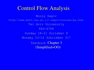
Data-Flow Analysis (Chapter 8). Mooly Sagiv. Outline. What is Data-Flow Analysis? Structure of an optimizing compiler An example: Reaching Definitions Basic Concepts: Lattices, Flow-Functions, and Fixed Points Taxonomy of Data-Flow Problems and Solutions Iterative Data-Flow Analysis

E N D
Data-Flow Analysis(Chapter 8) Mooly Sagiv
Outline • What is Data-Flow Analysis? • Structure of an optimizing compiler • An example: Reaching Definitions • Basic Concepts: Lattices, Flow-Functions, and Fixed Points • Taxonomy of Data-Flow Problems and Solutions • Iterative Data-Flow Analysis • Structural Data-Flow Analysis • DU-Chains and SSA
Data-Flow Analysis • Input: A control flow graph • Output:A control flow graph with “global” information at every basic blockExamples • Constant expressions: x+y*z • Live variables
Compiler Structure String of characters Scanner tokens Parser Symbol table and access routines OS Interface AST Semantic analyzer IR Code Generator Object code
Optimizing Compiler Structure String of characters Front-End IR Control Flow Analysis CFG Data Flow Analysis CFG+information Program Transformations Object code IR instruction selection
An Example Reaching Definitions • A definition --- an assignment to variable • An assignment d reaches a basic block if there exists an execution path to the basic block in which the value assigned at d is still active at the basic block
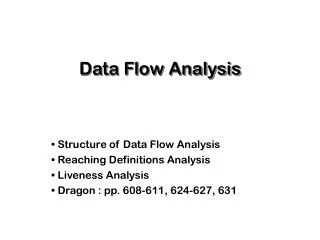
Running Example unsigned int fib(unsigned int m) {unsigned int f0=0, f1=1, f2, i; if (m <= 1) { return m; } else { for (i=2, i <=m, i++) { f2=f0+f1; f0=f1; f1 =f2;} return f2; } } 1: receive m(val) 2: f0 0 3: f1 1 4: if m <= 1 goto L3 5: i 2 6: L1: if i <=m goto L2 7: return f2 8: L2: f2 f0 + f1 9: f0 f1 10: f1 f2 11: i i + 1 12: goto L1 13: L3: return m
entry 1: receive m(val) 2: f0 0 3: f1 1 4: if m <= 1 goto L3 5: i 2 6: L1: if i <=m goto L2 7: return f2 8: L2: f2 f0 + f1 9: f0 f1 10: f1 f2 11: i i + 1 12: goto L1 13: L3: return m 2,3 2,3, 5,8,9, 10, 11 2,3, 5, 8,9, 10, 11 2,3, 5, 8,9, 10, 11 2,3, 5,8,9, 10, 11 2,3 exit
Difficulties in Data-Flow Analysis • Input-dependent information • Undecidability of program analysis • Reachability of basic blocks • Arithmetic • ...
1 int g(int m, int i) 2 int f(int n) 3 { int i=0; 4 if (n == 1) i = 2 5 while (n > 0) { 6 j = i+1; 7 n = g(n, i); 8 } 9 return j 10 }
Conservative data-flow analysis • Every piece of data-flow information is sound • Every enabled optimization is correct • A superset of the execution sequences is considered • In the reaching definition example a superset of the reaching definitions is computed
1 int g(int m, int i) 2 int f(int n) 3 { int i=0; 4 if (n == 1) i = 2 5 while (n > 0) { 6 j = i+1; 7 n = g(n, i); 8 } 9 return j 10 }
Iterative Computation of Reaching Definitions • Optimistically assume that at every block no definition is reached • Every basic block “generates” new definitions and “preserves” other definitions • No definition reaches ENTRY • Accumulate reaching definitions along different paths • Iteratively compute more and more definitions at every basic block • The process must terminate • The final solution is unique and conservative
Iterative Computation of Reaching Definitions RCin(ENTRY) = RCin(B) = B’ Pred(B) RCout(B’) RCout(B) = GEN(B) (RCin(B)PRSV(B))
entry 1: receive m(val) 2: f0 0 3: f1 1 4: if m <= 1 goto L3 5: i 2 6: L1: if i <=m goto L2 7: return f2 8: L2: f2 f0 + f1 9: f0 f1 10: f1 f2 11: i i + 1 12: goto L1 13: L3: return m 2,3 2,3, 5,8,9, 10, 11 2,3, 5, 8,9, 10, 11 2,3, 5, 8,9, 10, 11 2,3, 5,8,9, 10, 11 2,3 exit
Iterative Computation of Reaching Definitions Using Bit-Vectors • Represent every definition with a bit • PRSV and GEN are bit-vectors RCin(ENTRY) = <000...0> RCin(B) = B’ Pred(B) RCout(B’) RCout(B) = GEN(B) (RCin(B) PRSV(B))
entry 1: receive m(val) 2: f0 0 3: f1 1 4: if m <= 1 goto L3 5: i 2 6: L1: if i <=m goto L2 7: return f2 8: L2: f2 f0 + f1 9: f0 f1 10: f1 f2 11: i i + 1 12: goto L1 13: L3: return m 2,3 2,3, 5,8,9, 10, 11 2,3, 5, 8,9, 10, 11 2,3, 5, 8,9, 10, 11 2,3, 5,8,9, 10, 11 2,3 exit
Complete Join-Lattices • A set L of “data-flow” information • A partial order on the elements of L • x y x “covers” less states than y x is more precise than y • is the minimum element • height of a lattice length of maximal strictly increasing chain x1x2... xk • A “join” confluence operator : LLL • x xy, y xy • x z, y z xy z • Examples: Powersets, Bit-Vectors, ICP
Properties of Lattices • x = x = x • x x = x (reflexivity) • x y = y x (commutativity) • (x y ) z = x (y z) (associativity)
Functions on Lattices • Models effects of basic blocks • A monotonic function f: L L x y f(x) f(y) • A distributive function f: L L f(x) f(y) = f(x y) • A fixed point of a function f, f(x) = x • For a monotonic function f the effective height of L w.r.t. f, the longest increasing chainf()f2()=f(f())... fk() = lfp(f)
The Join (Meet) Over All Paths • A data-flow solution which is precise under the assumption that every control flow path is executable • For a path [B1, B2, ... Bn] Fp = FBn ... FB2FB1 • The JOP at a block BJOP(B) = P Path(B) Fp(Init) • For distributive Fp compute JOP • Otherwise, find X(B) JOP(B)
entry w > 0? N Y u 1 v 2 u 2 v 1 w u+v exit
Dimensions for Data-Flow Problems • The information provided • “ralational” Vs. independent attributes • The type of lattice and functions usedpowersets, ICP, ..., unbounded heights • The direction of information flowforward, backward, bidirectional
Example Data-Flow Problems • Reaching Definitions • Available Expressions • Live Variables • Upward Exposed Uses • Copy-Propagation Analysis • Constant-Propagation Analysis • Partial-Redundency Analysis
entry z > 1? N Y x 1 z > y x 2 N Y z x-3 y x+1 exit
Data-Flow Analysis Algorithms • Allen’s strongly connected regions • Kildall’s iterative algorithm • Ullman’s T1-T2 analysis • Kennedy’s node-listing algorithm • Farrow, Kennedy, and Zuconi’s graph grammar approach • Rosen’s high-level approach • structural analysis • slotwise analysis
Iterative Data-Flow Analysis in(ENTRY) = Init In(B) = B’ Pred(B) Out(B’) Out(B) = FB(In(B))
Iterative Data-Flow Algorithm Input:aflow graph G=(N,E,r) An init value Init A montonic function FB for every B in N Output:For every N in(N) Initializatio: in(Entry) := Init; for each node B in N-{Entry} do in(B) := WL := N - {Entry} Iteration: while WL != {} do Select and remove an B from WL out := FB(in(B)) For all B’ in succ(B) such that in(B’) != in(B’) out do in(B’):= in(B’) out WL := WL {B’}
Post-ordering Input:aflow graph G=(N,E,r) Output:a depth-first spanning tree (N,T) andordering Post ofN Method:T := Ø; for each node n in N do mark n unvisited; i := 1; call DFS(r) Using:procedure DFS(n) is mark n visited; for each n ® s in E doif s is not visited then add the edge n ® s to T; call DFS(s); Post(n) := i; i := i + 1;
entry 8 1: receive m(val) 2: f0 0 3: f1 1 4: if m <= 1 goto L3 5: i 2 6: L1: if i <=m goto L2 7: return f2 8: L2: f2 f0 + f1 9: f0 f1 10: f1 f2 11: i i + 1 12: goto L1 13: L3: return m 7 6 5 3 4 1 2 exit
entry 1 1: receive m(val) 2: f0 0 3: f1 1 4: if m <= 1 goto L3 5: i 2 6: L1: if i <=m goto L2 7: return f2 8: L2: f2 f0 + f1 9: f0 f1 10: f1 f2 11: i i + 1 12: goto L1 13: L3: return m {} {} 2 {2, 3} 3 {2, 3, 5} 4 {2, 3, 5} 6 {2, 3, 5} 5 8 {2, 3} 7 exit
entry 1 1: receive m(val) 2: f0 0 3: f1 1 4: if m <= 1 goto L3 5: i 2 6: L1: if i <=m goto L2 7: return f2 8: L2: f2 f0 + f1 9: f0 f1 10: f1 f2 11: i i + 1 12: goto L1 13: L3: return m {} {} 2 {2, 3} 3 {2, 3, 5, 8, 9, 10} 4 {2, 3, 5} 6 {2, 3, 5} 5 8 {2, 3} 7 exit
entry 1 1: receive m(val) 2: f0 0 3: f1 1 4: if m <= 1 goto L3 5: i 2 6: L1: if i <=m goto L2 7: return f2 8: L2: f2 f0 + f1 9: f0 f1 10: f1 f2 11: i i + 1 12: goto L1 13: L3: return m 2 {2, 3} 3 {2, 3, 5, 8, 9, 10} 4 6 {2, 3, 5, 8, 9, 10} {2, 3, 5, 8, 9, 10} 5 8 {2, 3} 7 exit
entry 1 1: receive m(val) 2: f0 0 3: f1 1 4: if m <= 1 goto L3 5: i 2 6: L1: if i <=m goto L2 7: return f2 8: L2: f2 f0 + f1 9: f0 f1 10: f1 f2 11: i i + 1 12: goto L1 13: L3: return m 2 {2, 3} 3 {2, 3, 5, 8, 9, 10} 4 6 {2, 3, 5, 8, 9, 10} {2, 3, 5, 8, 9, 10} 5 {2, 3, 5, 8, 9, 10} 8 {2, 3} 7 exit
Iterative Backward Data-Flow Analysis Out(Exit) = Init Out(B) = B’ Succ(B) In(B’) In(B) = FB(Out(B))
Lattices of Flow Functions • For a lattice L LF are the montonic functions from L to L f LF x y f(x) f(y) • LF is a lattice with the order f g for all z: f(z) g(z) • F(z) • (x F y)(z) x(z) y(z) • LF is closed under composition (f g)(z) f(g(z)) • f0id, fn f fn-1 • f*(z)limn (id f)n (z)
Structural Data-Flow Analysis • Phase 1: Compute “the effect” of every program construct in a bottom-up fashion on the tree of control flow constructs(control-tree) • Phase 2: Propagates the data-flow value in a top-down fashion into basic blocks
if Fif/Y Fif/N then if-then Fif-then Fthen Bottom-Up Phase(if-then) Fif-then=(F then° Fif/Y) Fif/N
if Fif Fif then if-then Fif-then Fthen Bottom-Up Phase(Simplified if-then) Fif-then=(F then° Fif) Fif
if FG1, P1 FG1, P1 then if-then FG, P FG2, P2 Bottom-Up PhaseReaching Definitions(Simplified if-then) (F G2, P2° FG1, P1) FG1, P1 F (G1P2)G2, P1 P2 FG1, P1 F G1G2, P1
if Fif/Y Fif/N then if-then Fif-then Fthen Top-Down Phase(if-then) in(if-then)=in(if) in(then) = Fif/Y(in(if))
if Fif Fif then if-then Fif-then Fthen Top-Down Phase(Simplified if-then) in(if-then)=in(if) in(then) = Fif (in(if))
if FG1, P1 FG1, P1 then if-then FG,P FG2, P2 Top-Down PhaseReaching Definitions(Simplified if-then) in(if) = in(if-then) in(then) = FG1, P1 (in(if))
if Fif/Y Fif/N if-then-else then else Fif-then-else Fthen Felse Bottom-Up Phase(if-then-else) Fif-then-else=(F then° Fif/Y) (F else° Fif/N)
if Fif Fif if-then-else then else Fif-then-else Fthen Felse Bottom-Up Phase(simplified if-then-else) Fif-then-else=(F then° Fif) (F else° Fif)= =(F then F else )° Fif
if FG0, P0 FG0, P0 if-then-else then else FG,P FG1,P1 FG2, P2 Bottom-Up Phase Reaching Definitions(simplified if-then-else) (F G1, P1 F G2, P2 )° FG0, P0 F G1G2, P1P2, ° FG0, P0 F(G0 (P1P2)) G1G2, P0 (P1P2)
if Fif/Y Fif/N if-then-else then else Fif-then-else Fthen Felse Top-Down Phase(if-then-else) in(if)=in(if-then-else) in(then)= Fif/Y (in(if)) in(else)= Fif/N (in(if))
if Fif Fif if-then-else then else Fif-then-else Fthen Felse Top-Down Phase(Simplified if-then-else) in(if)=in(if-then-else) in(then)= Fif (in(if)) in(else)= Fif (in(if))
if FG0, P0 FG0, P0 if-then-else then else FG,P FG1,P1 FG2, P2 Top-Down-Up Phase Reaching Definitions(simplified if-then-else) in(if)=in(if-then-else) in(then)= FG0, P0 (in(if)) in(else)= FG0, P0 (in(if))
while Fwhile/Y while-loop body Fwhile-loop Fbody Bottom-Up Phase(while) Fwhile-loop=Fwhile/N °(F body° Fwhile/Y)* Fwhile/N