Download
1 / 19
200 likes | 503 Vues
Data Flow Analysis. Structure of Data Flow Analysis Reaching Definitions Analysis Liveness Analysis Dragon : pp. 608-611, 624-627, 631. Data Flow Analysis. Local data Flow Analysis (e.g., value numbering) Analyze effect of each instruction

E N D
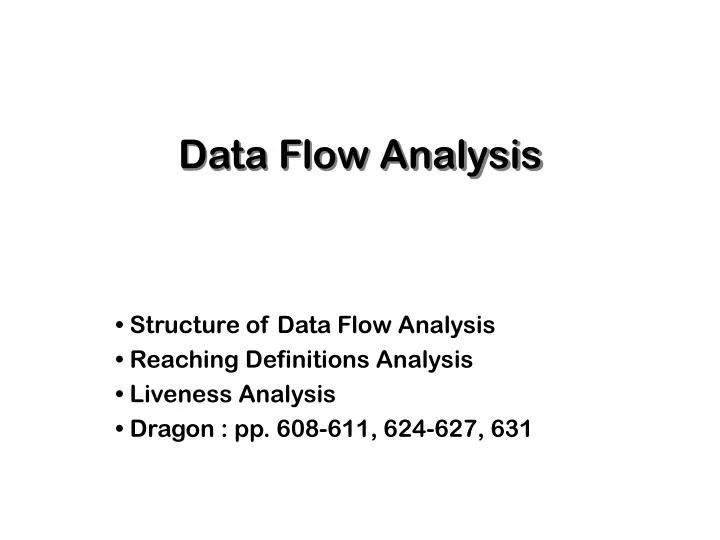
Data Flow Analysis Structure of Data Flow Analysis Reaching Definitions Analysis Liveness Analysis Dragon : pp. 608-611, 624-627, 631
Data Flow Analysis • Local data Flow Analysis (e.g., value numbering) • Analyze effect of each instruction • Compose effects of instructions to derive information from beginning of basic block to each instruction • Global Data Flow Analysis • Analyze effect of each basic block • Compose effects of basic blocks to derive information at basic block boundaries • From basic block boundaries, apply local technique to generate information on instructions (You can also do global analysis in the level of instructions, yet it would be more expensive)
Effects of a Basic Block • Effects of an instruction : a = b + c • Uses variables b and c • Kills an old definition of a • Generate a new definition a
Compose effects of instructions : Effect of a basic block • A locally exposed use in a BB is a use of a data item which is not preceded in the BB by a definition of the data item • Any definition of a data item in the BB kills all definitions of the same data item reaching the BB • A locally generated definition : last definition of data item in BB • t1 = r1 + r1 • r2 = t1 • t2 = r2 + r1 • r1 = t2 • t3 = r1 * r2 • r2 = t3 • if r2 > 100 goto L1
Across Basic Blocks • Static Program vs. Dynamic Execution • Statically : finite program • Dynamically : potentially infinite possible execution paths Can reason about each possible path as if all instructions executed are in one BB • Data Flow Analysis • Associate with each static point in the program information true of the set of dynamic instances of that program point
Reaching Definition • A definition of a variable x is an instruction that assigns, • or may assign, a value to x • A definitiond reaches a point p if there exists a path from the point immediately following d to p such that d is not killed along that path
Problem Statement • For each basic block b, determine if each definition in the program reaches b • A representation • IN[B], OUT[B] : a bit vector, one bit for each definition
Describing Effects of the Nodes (basic blocks) A transfer functionfb for a basic block b : OUT[b] = fb(IN[b]) (incoming reaching definitions outgoing reaching definitions
A basic block b • generates definitions : GEN[b], set of locally generated definitions in b • propagate definitions : IN[b] - KILL[b], where KILL[b] is set of definitions in rest of program killed by definitions in b • OUT[b] = GEN[b] ( IN[b] - KILL[b] )
Effects of Edges (Acyclic) • OUT[b] =fb(IN[b]) • Join node : a node with multiple predecessors • meet operator : IN[b] = OUT[p1] OUT[p2] … OUT[pn] , where p1 , p2, …, pn are all predecessors of b
Cyclic Graphs • Equations still hold • OUT[b] =fb(IN[b]) • IN[b] = OUT[p1] OUT[p2] … OUT[pn] • Solve for fixed point solution
Reaching Definitions : Worklist Algorithm Input : control Flow Graph CFG = ( N, E, Entry, Exit ) /* Initialize */ OUT[Entry] = { } for all nodes i OUT[i] = { } ChangeNodes = N /* Iterate */ while ChangeNodes != { } { Remove i from ChangeNodes IN[i] = U (OUT[p]), for all predecessors p of i oldout = OUT[i] OUT[i] = f_i(IN[i]) /* OUT[i] = GEN[i] U (IN[i] - KILL[i]) */ if (oldout != OUT[i]) { for all successors s of i add s to ChangeNodes } }
entry d1 : i = m -1 d2 : j = n d3 : a = u1 d4 : i = i + 1 d2 : j = j - 1 d4 : i = i + 1 d2 : j = j - 1 d6 : a = u2 d7 : i = u3 exit Example
Live Variable Analysis • Definition • A variable v is live at point p if the value of v is used along some path in the flow graph starting at p • Otherwise, the variable is dead • Problem • For each basic block, determine if each variable is live in each basic block • Size of bit vector : one bit for each variable
Effects of a Basic Block • Observation : Trace uses back to the definitions • A basic block b can • generate live variables : USE[b], set of locally exposed uses in b • Propagate incoming live variables : OUT[b] - DEF[b], where DEF[b] is set of variables defined in b • Transfer functions for block b • IN[b] = USE[b] ( OUT[b] - DEF[b] )
Flow Graph • IN[b] =fb(OUT[b]) • Join node : a node with multiple successors • meet operator : OUT[b] = IN[s1] IN[s2] … IN[sn] , where s1 , s2, …, sn are all successors of b
Live Variable : Worklist Algorithm Input : control Flow Graph CFG = ( N, E, Entry, Exit ) /* Initialize */ IN[Entry] = { } for all nodes i IN[i] = { } ChangeNodes = N /* Iterate */ while ChangeNodes != { } { Remove i from ChangeNodes IN[i] = U (OUT[s]), for all predecessors s of i oldin = IN[i] IN[i] = f_i(OUT[i]) /* IN[i] = USE[i] U (OUT[i] - DEF[i]) */ if (oldout != IN[i]) { for all predecessors p of i add p to ChangeNodes } }
entry d1 : i = m -1 d2 : j = n d3 : a = u1 d4 : i = i + 1 d2 : j = j - 1 d4 : i = i + 1 d2 : j = j - 1 d6 : a = u2 d7 : i = u3 exit Example