Download
1 / 1
10 likes | 93 Vues
SYNTHETIC RAINFALL SERIES GENERATION - MDM Heinz D. Fill , André F. Santana, Miriam Rita Moro Mine Contacts: mrmine.dhs@ufpr.br. 1. MONTHLY DISAGGREGATION MODEL - DUM

E N D
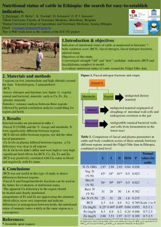
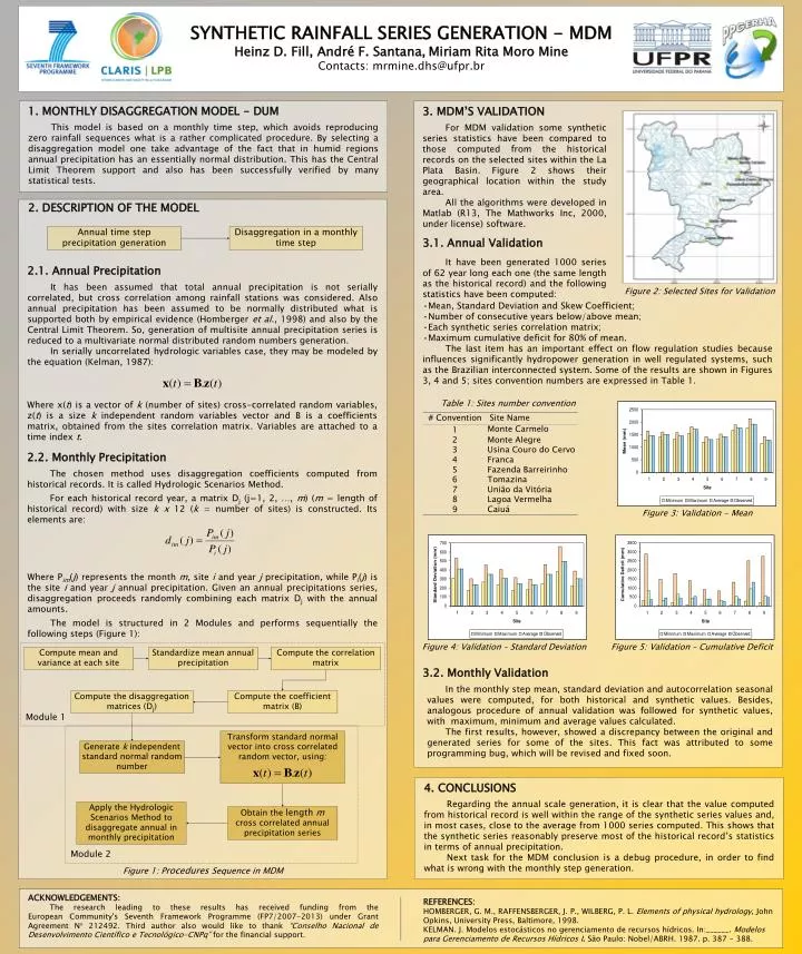
SYNTHETIC RAINFALL SERIES GENERATION - MDM Heinz D. Fill, André F. Santana,Miriam Rita Moro Mine Contacts: mrmine.dhs@ufpr.br 1. MONTHLY DISAGGREGATION MODEL - DUM This model is based on a monthly time step, which avoids reproducing zero rainfall sequences what is a rather complicated procedure.By selecting a disaggregation model one take advantage of the fact that in humid regions annual precipitation has an essentially normal distribution. This has the Central Limit Theorem support and also has been successfully verified by many statistical tests. 3. MDM’S VALIDATION For MDM validation some synthetic series statistics have been compared to those computed from the historical records on the selected sites within the La Plata Basin. Figure 2 shows their geographical location within the study area. All the algorithms were developed in Matlab (R13, The Mathworks Inc, 2000, under license) software. 3.1. Annual Validation It have been generated 1000 series of 62 year long each one (the same length as the historical record) and the following statistics have been computed: 2. DESCRIPTION OF THE MODEL Annual time step precipitation generation Disaggregation in a monthly time step 2.1. Annual Precipitation It has been assumed that total annual precipitation is not serially correlated, but cross correlation among rainfall stations was considered. Also annual precipitation has been assumed to be normally distributed what is supported both by empirical evidence (Homberger et al., 1998) and also by the Central Limit Theorem. So, generation of multisite annual precipitation series is reduced to a multivariate normal distributed random numbers generation. In serially uncorrelated hydrologic variables case, they may be modeled by the equation (Kelman, 1987): Figure 2: Selected Sites for Validation • Mean, Standard Deviation and Skew Coefficient; • Number of consecutive years below/above mean; • Each synthetic series correlation matrix; • Maximum cumulative deficit for 80% of mean. • The last item has an important effect on flow regulation studies because influences significantly hydropower generation in well regulated systems, such as the Brazilian interconnected system. Some of the results are shown in Figures 3, 4 and 5; sites convention numbers are expressed in Table 1. Where x(t) is a vector of k (number of sites) cross-correlated random variables, z(t) is a size k independent random variables vector and B is a coefficients matrix, obtained from the sites correlation matrix. Variables are attached to a time index t. 2.2. Monthly Precipitation The chosen method uses disaggregation coefficients computed from historical records. It is called Hydrologic Scenarios Method. For each historical record year, a matrix Dj (j=1, 2, …, m) (m = length of historical record) with size k x 12 (k = number of sites) is constructed. Its elements are: Table 1: Sites number convention Figure 3: Validation - Mean Where Pim(j) represents the month m, site i and year j precipitation, while Pi(j) is the site i and year j annual precipitation. Given an annual precipitations series, disaggregation proceeds randomly combining each matrix Dj with the annual amounts. The model is structured in 2 Modules and performs sequentially the following steps (Figure 1): Figure 4: Validation – Standard Deviation Figure 5: Validation – Cumulative Deficit Compute mean and variance at each site Standardize mean annual precipitation Compute the correlation matrix • 3.2. Monthly Validation • In the monthly step mean, standard deviation and autocorrelation seasonal values were computed, for both historical and synthetic values. Besides, analogous procedure of annual validation was followed for synthetic values, with maximum, minimum and average values calculated. • The first results, however, showed a discrepancy between the original and generated series for some of the sites. This fact was attributed to some programming bug, which will be revised and fixed soon. Compute the disaggregation matrices (Dj) Compute the coefficient matrix (B) Module 1 Transform standard normal vector into cross correlated random vector, using: Generate k independent standard normal random number 4. CONCLUSIONS Regarding the annual scale generation, it is clear that the value computed from historical record is well within the range of the synthetic series values and, in most cases, close to the average from 1000 series computed. This shows that the synthetic series reasonably preserve most of the historical record’s statistics in terms of annual precipitation. Next task for the MDM conclusion is a debug procedure, in order to find what is wrong with the monthly step generation. Apply the Hydrologic Scenarios Method to disaggregate annual in monthly precipitation Obtain the length mcross correlated annual precipitation series Module 2 Figure 1: ProceduresSequence in MDM ACKNOWLEDGEMENTS: The research leading to these results has received funding from theEuropean Community's Seventh Framework Programme (FP7/2007-2013) under Grant Agreement N° 212492.Third author also would like to thank “Conselho Nacional de Desenvolvimento Científico e Tecnológico-CNPq” for the financial support. REFERENCES: HOMBERGER, G. M., RAFFENSBERGER, J. P., WILBERG, P. L. Elements of physical hydrology, John Opkins, University Press, Baltimore, 1998. KELMAN. J. Modelos estocásticos no gerenciamento de recursos hídricos. In:______. Modelos para Gerenciamento de Recursos Hídricos I. São Paulo: Nobel/ABRH. 1987. p. 387 - 388.