Download
1 / 39
390 likes | 392 Vues
This lecture explores the fundamentals of projection in linear algebra and functional analysis, highlighting its importance in various scientific computing applications. Topics covered include sparse matrices, parallel implementations, numerical solution of PDEs, and iterative methods.

E N D
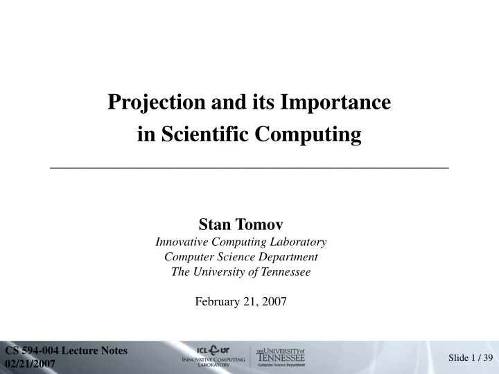
Projection and its Importance • in Scientific Computing • ________________________________________________ Stan Tomov Innovative Computing Laboratory Computer Science Department The University of Tennessee February 21, 2007 CS 594-004 Lecture Notes 02/21/2007
Contact information office : Claxton 330 phone : (865) 974-6317 email : tomov@cs.utk.edu • Additional reference materials:[1] R.Barrett, M.Berry, T.F.Chan, J.Demmel, J.Donato, J. Dongarra, V. Eijkhout, R.Pozo, C.Romine, and H.Van der Vorst, Templates for the Solution of Linear Systems: Building Blocks for Iterative Methods (2nd edition) http://netlib2.cs.utk.edu/linalg/html_templates/Templates.html • [2] Yousef Saad, Iterative methods for sparse linear systems (1st edition)http://www-users.cs.umn.edu/~saad/books.html
Topics Projection inScientific Computing(lecture 1) Sparse matrices, parallel implementations(lecture 3, 03/21/07) PDEs, Numerical solution, Tools, etc. (lecture 2, 02/28/07) Iterative Methods (lectures 4 and 5, 04/11 and 04/18/07)
Outline • Part I • Fundamentals • Part II • Projection in Linear Algebra • Part III • Projection in Functional Analysis (e.g. PDEs)
What is Projection? • Here are two examples (from linear algebra) (from functional analysis) u u = f(x) Pu 1 e = 1 Pu e 0 1 P : orthogonal projection of vector u on e P : best approximation (projection) of f(x) in span{ e } ⊂ C[0,1]
Definition • Projection is a linear transformation P from a linear space V to itself such that P2 = PequivalentlyLet V is direct sum of subspaces V1 and V2 V = V1 V2i.e. for u ∈ V there are unique u1∈ V1 and u2∈V2 s.t. u = u1+u2Then P: VV1 is defined for u ∈ V as Pu ≡ u1
Importance in Scientific Computing • To compute approximations Pu u where dim V1 << dim VV = V1 V2 • When computation directly in V is not feasible or even possible.A few examples: • Interpolation (via polynomial interpolation/projection) • Image compression • Sparse iterative linear solvers and eigensolvers • Finite Element/Volume Method approximations • Least-squares approximations, etc.
Projection in R2 • In R2 with Euclidean inner-product, i.e. for x, y ∈ R2(x, y) = x1 y1 + x2 y2 ( = yT x = x⋅y ) and || x || = (x, x)1/2 u (u, e) Pu = e (Exercise) || e ||2 e e i.e. for || e || = 1 Pu = (u, e) e Pu P : orthogonal projection of vector u on e
Projection in Rn / Cn • Similarly to R2P : Orthogonal projection of u into span{e1, ... , em}, m ≤ n. Let ei, i = 1 ... m is orthonormal basis, i.e. (ei, ej) = 0 for i≠j and (ei, ej) = 1 for i=jP u = (u, e1) e1 + ... + (u, em) em ( Exercise ) Orthogonal projection of u on e1
How to get an orthonormal basis? • Can get one from every subspace by Gram-Schmidt orthogonalization:Input : m linearly independent vectors x1, ..., xmOutput : m orthonormal vectors x1, ..., xm 1. x1 = x1 / || x1 || 2. do i = 2, m 3. xi = xi - (xi, x1) x1 - ... - (xi, xi-1) xi-1 (Exercise: xi x1 , ... , xi-1) 4. xi = xi / || xi || 5. enddoKnown as Classical Gram-Schmidt (CGM) orthogonalization Orthogonal projection of xi on x1
How to get an orthonormal basis? • What if we replace line 3 with the following (3')? 3. xi = xi - (xi, x1) x1 - ... - (xi, xi-1) xi-1 3'. do j = 1, i-1 xi = xi – (xi, xj) xj enddo • Equivalent in exact arithmetic (Exercise) but not with round-off errors (next) ! • Known as Modified Gram-Schmidt (MGS) orthogonalization xi
CGS vs MGS CGS vs MGS Results from Julien Langou:Scalability of MGS and CGS on two different clusters for matrices of various size
CGS vs MGS Results from Julien Langou:Accuracy of MGS vs CGS on matrices of increasing condition number
QR factorization • Let A = [x1, ... , xm] be the input for CGS/MGS and Q = [q1, ... , qm] the output;R : an upper m m triangular matrix defined from the CGR/MGS. ThenA = Q R
Other QR factorizations • What about the following? 1. G = ATA 2. G = L LT (Cholesky factorization) 3. Q = A (LT)-1 • Is Q orthonormal, i.e. A = QLT to be a QR factorization (Exercise) • When is this feasible and how compares to CGS and MGS?
Other QR factorizations • Feasible when n >> m • Allows efficient parallel implementation:blocking both computation and communication AT A G = In accuracy is comparable to MGS In scalability is comparable to CGSExercise P1 P2 . . .
How is done in LAPACK? x w • Using Householder reflectors H = I – 2 w wT • w = ? so that H x1 = e1 w = ... (compute or look at the reference books) • Allows us to construct Xk Hk-1 ... H1 X = Hx Q(Exercise) LAPACK implementation : “delayed update” of the trailing matrix + “accumulate transformation” to apply it as BLAS 3
Part II Projection in Linear Algebra
Projection into general basis • How to define projection without orthogonalization of a basis? • Sometimes is not feasible to orthogonalize • Often the case in functional analysis(e.g. Finite Element Method, Finite Volume Method, etc.) where the basis is “linearly independent” functions (more later, and Lecture 2) • We saw if X = [x1, ... , xm] is an orthonormal basis (*) P u = (u, x1) x1 + ... + (u, xm) xm • How does (*) change if X are just linearly independent ?P u = ?
Projection into a general basis • The problem:Find the coefficients C = (c1 ... cm)T in P u = c1 x1 + c2 x2 + . . . + cm xm = X C so that u – Pu ⊥ span{x1, ..., xm}or ⇔ so that the error e in (1) u = P u + eis ⊥ span{x1, ..., xm}
Projection into a general basis • (1)u = P u + e = c1 x1 + c2 x2 + . . . + cm xm + e • Multiply (1) on both sides by “test” vector/function xj(terminology from functional analysis) for j = 1,..., m(u , xj) = c1 (x1 , xj)+ c2 (x2 , xj)+ . . . + cm (xm , xj) + (e, xj) • i.e. m equations for m unknowns • In matrix notations (XT X) C = XT u (Exercise) XT Pu = XT u • XTX is the so called Gram matrix (nonsingular; why?) 0
Normal equations • System(XT X) C = XT uis known also as Normal Equations • Can be solved using the Method of Normal Equations from slide # 16 (with the Cholesky factorization)
Least Squares (LS) • System(XTX) C = XTugives also the solution of the LS problem min || X C – u ||since || v1 – u ||2 = || (v1 – Pu) – e ||2 = || v1 – Pu ||2 + || e ||2≤ || e ||2 = || Pu – u ||2 for ∀ v1∈ V1 P u C∈Rm
LS • Note that the usual notations for LS is: For A∈Rnm, b∈Rn findmin || A x – b || • Solving LS with QR factorization Let A = Q R, QTA = R = R1 , QT b =cm0 d n - m Then || Ax – b ||2 = || QTAx – QTb ||2 = || R1x – c ||2 + || d ||2 i.e. we get minimum if x is such that R1 x = c x∈Rm
Projection and iterative solvers • The problem : Solve Ax = b in Rn • Iterative solution: at iteration i extract an approximatexi from just a subspace V = span[v1, ..., vm] of Rn • How? As on slide 22, impose constraints: b – Ax subspace W = span[w1,...,wm] of Rn, i.e. (*) (Ax, wi) = (b, wi) for ∀ wi∈W= span[w1,...,wm] • Conditions (*) known also as Petrov-Galerkin conditions • Projection isorthogonal: V and W are the same (Galerkin conditions) oroblique : V and W are different
Matrix representation • Let V = [v1, ..., vm], W = [w1,...,wm] Find y ∈Rm s.t. x = x0 + V ysolves Ax = b, i.e.A V y = b – Ax0 = r0subject to the orthogonality constraints:WTA V y = WT r0 • The choice for V and W is crucial and determines various methods (more in Lectures 4 and 5)
A General Projection Algorithm • Prototype from Y.Saad's book
Projection and Eigen-Solvers • The problem : Solve Ax = x in Rn • As in linear solvers: at iteration i extract an approximatexi from a subspace V = span[v1, ..., vm] of Rn • How? As on slides 22 and 26, impose constraints:x – Ax subspace W = span[w1,...,wm] of Rn, i.e. (*) (Ax, wi) = (x, wi) for ∀ wi∈W= span[w1,...,wm] • This procedure is known as Rayleigh-Ritz • Again projection can beorthogonal or oblique
Matrix representation • Let V = [v1, ..., vm], W = [w1,...,wm] Find y ∈Rm s.t. x = V ysolves Ax = x, i.e.A V y = Vysubject to the orthogonality constraints:WTA V y = WT Vy • The choice for V and W is crucial and determines various methods (more in Lectures 4 and 5)
Projection in Functional Spaces • The discussion so far can be applied to any functional inner-product space (examples to follow) • An important space is C[a, b], the space of continuous functions on [a, b], with inner-product a (f, g) = ∫f(x) g(x) dx band induced norm || f || = (f, f)1/2
Projection in Functional Spaces • Projection P: V V1 where V = V1 V2 • In functional analysis and scientific computing V1 is usually taken as • Piecewise polynomials • In PDE approximation (FEM/FVM), Numerical integration, etc. • Trigonometric functions { sin(n x), cos(n x) }n=0,... , x [0, 2]Orthogonal relative to 2 (f, g) = ∫f(x) g(x) dx (Exercise)0
Normal equations / LS • Exercise: f(x) = sin(x)Find the projection in V1 = span{x, x3, x5} on interval [-1, 1] using inner-product 1(f, g) = ∫f(x) g(x) dx -1and norm || f || = (f,f)1/2
Normal equations / LS • Leads to Gram matrix that is very ill-conditioned(called Hilbert matrix: Gram matrix for polynomials 1, x, x2, x3, ...) • For numerical stability is better to orthogonalize the polynomials • There are numerous examples of orthonormal polynomial sets* Legendre, Chebyshev, Hermite, etc * Check the literature for more if interested
Integration via Polynomial Interpolation • Take∫f(x) dx ∫p(x) dx where p is a polynomial approximation to f • Taking p a polynomial interpolating f at n+1 fixed nodes xi leads to quadrature formulas∫f(x) dx A0 f(x0) + ... + An f(xn) that are exact exact for polynomials of degree ≤ n • Smart choice of the nodes xi (Gaussian quadrature) leads to formulas that are exact for polynomials of degree ≤ 2n+1
Galerkin Projection • Numerical PDE discretizations have a common concept: • Represent computational domain with mesh • Approximate functions and operators over the mesh
Galerkin Projection i • Finite dimensional spaces (e.g. V1) cancan be piecewise polynomialsdefined over the mesh, e.g. • Numerical solution of PDE (e.g. FEM) • Boundary value problem: Au = f, subject to boundary conditions • Get a “weak” formulation: (Au, ) = (f, ) - multiply by test function and integrate over the domain a( u, ) = <f, > for S • Galerkin (FEM) problem: Find uh Sh S s.t. a( uh, h) = <f, h> for hSh i
Learning Goals • The idea and application of Petrov-Galerkin conditions as a way of defining computationally feasible/possible formulations (approximations) • Some generic examples demonstrating from • Linear algebra • Functional analysis (to get more specific in the following lectures)