Download
1 / 29
290 likes | 293 Vues
Folding@Home: Pushing the boundaries of atomistic simulation with world-wide grid computing. Vijay Pande Stanford University. Why simulate folding?. Experiments are not enough Timescales are very fast (experiments difficult) We want atomic detail

E N D
Folding@Home:Pushing the boundaries of atomistic simulation with world-wide grid computing Vijay Pande Stanford University
Why simulate folding? • Experiments are not enough • Timescales are very fast (experiments difficult) • We want atomic detail • Experiments ensemble average significantly – a problem? • Protein folding as a paradigm for other tough problems • The issues relevant for simulating protein folding will be important in many other areas • Protein-protein interactions, protein design, ligand binding Unfolded conformers Folded (“native”) tertiary structure
Goals for biophysical simulation • Quantitative agreement with experiment • Real numbers, statistics, etc are important • Forcefields, etc are still not proven • Unbiased simulation • Don’t build in the answer (no native state knowledge) • True predictive capability • A simple, physically-based method • Easy to understand and analyze, limitations clear • Gain insight, not just reproduce experiments • Can we learn something that wasn’t obvious before?
Range of possible models Great sampling Accurate model Off-lattice models: simple models of particular proteins Lattice models: simple & generic All-atom models: very detailed, typically intractable CPU minute CPU hour 1000 CPU years
MD step long MD run where we need to be where we’d love to be Relevant timescales Bond vibration Isomer- ation Water dynamics Helix forms Fastest folders typical folders slow folders 10-15 femto 10-12 pico 10-9 nano 10-6 micro 10-3 milli 100 seconds • Fundamental problem for simulation • Proteins fold in micro- to milliseconds • Computers can simulate nanoseconds • How can we break this impasse?
Traditional approach: Use many processors to speed a single calculation • How? Divide the force calculation of a trajectory between CPUs • Spatial decomposition for work division • “computer science” approach • Has not simulated folding to date • Can 60 students work together to complete an hour exam in 1 minute? No. Scaling is hard. eg, Duan and Kollman, Science (1998) • Communication overwhelming Spatial decomposition divides real space among CPUs
Why is the dynamics so slow? • Folding is a free energy barrier crossing process • Spend most of the time dwelling in the unfolded state … • … until a lucky, thermal fluctuation comes along • Analogy to gas liquid transition • Formation of critical nucleus is rate limiting • Most time is spent waiting for a “lucky” thermal fluctuation • Let’s try to invent a “physical chemistry” approach
Can we use uncoupled trajectories to access long timescales? Barrier crossing is a stochastic process with exponential kinetics: let’s take advantage of this Fraction that cross: f(t) = 1 – exp(-kt) At short times, we get f(t) k t What if we run M Simulations in parallel each of time t? Mkt will cross f(t) = 1 – exp(-kt) f(t) k t Putting in real numbers: number that cross = Mkt = 10,000 simulations x 10,000ns-1 x 100ns = 100 events!
F vi U Pij vj å å s = × s = + MFPT P ( t MFPT ) P i ij ij j i ij j edge edge ij ij s s 0 , 1 = = = MFPT 0 I F F New method: build Markovian State Model (MSM) from a graph of trajectories • Build graph • use MD to determine transition probability • master equation for dynamics • Benefits • efficiently uses many short trajectories • can capture non-exponential kinetics Challenge: to build a Markovian representation of the state space Solution: clustering of conformations retains Markovian behavior • Iterative procedure to calculate kinetic properties MSFT = Mean First Passage Time ~ 1/k s = commitment probability = “pfold” Singhal, Snow, and Pande. Journal of Chemical Physics (2004)
Folding@Home:Worldwide desktop grid computing • Very powerful • ~200 Teraflops sustained performance • ~1,000,000 total CPUs, >150,000 active • >200 countries • Very low cost • $100,000 for server hardware & admin = $1/CPU/year • Supercomputer TCO ~$10,000/CPU/year • New paradigm for supercomputing • design algorithms touse many CPUs, slownetworking ~150,000 active CPUs over the world (CPU locations from IP address)
How we predict rates for single exponential kinetics Minimum time (2ns) Quick estimate: look at the slope of this plot, f(t) = kt (more complex: use maximum likelihood methods)
100000 villin BBAW 10000 Trp cage beta hairpin 1000 Predicted folding time (nanoseconds) 100 alpha helix 10 PPA 1 1 10 100 1000 10000 100000 experimental measurement (nanoseconds) Kinetics: predicted vs experiment(with several different experimental collaborators) • Purely physical model • only the protein sequence and laws of physics go into our model • no native state information used to generate trajectories • Quantitative comparison to experiment • absolute rates: no free parameters
How could proteins fold? • Form secondary structure first (Diffusion/Collision) • Hierarchical: form helices & hairpins, decrease entropy • Nucleation • Form nucleus of structure, then grow (ala 1st order phase trans) • Collapse first • Hydrophobically driven: remove water to form HBs • Form rough native shape first (topomer search) • Find the right “topology” first, then pack side chains Questions: • Do any proteins fold via these mechanisms? • Are any of these “universal” • Can simulations help to arbitrate?
BBA5 Folding in TIP3P • Reach native state • rate (4.5ms) agrees with experiment (7.5ms) • TIP3P corrected rate is 7.5ms • Methods • Amber94-GS, NPT, RF • 250 ms simulated time (>106 CPU-days on Folding@Home) (BBA5 designed and characterizedby Barbara Imperiali’s group)
TIP3P GB/SA Similarities in the folding mechanism: TIP3P vs GB/SA • Both TIP3P and GB/SA lead to a diffusion-collision mechanism • 2nd structure forms independently • probability of forming helix & hairpin statistically independent: P(helix & hairpin) = P(helix) P(hairpin)
How do proteins fold? • We find no single mechanism • Collapse first (protein G Hairpin) • Hydrophobically driven, must remove water in order to make hydrogen bonds stable • Form secondary structure first (BBA5) • Form helices & hairpins • Hierarchical, decrease in entropy • Form rough native shape first (Villin) • Are there any universal aspects? • So far, no! Perhaps there isn’t anything to find? • Evolution uses what ever works
100000 villin BBAW 10000 Trp cage beta hairpin 1000 Predicted folding time (nanoseconds) 100 alpha helix 10 PPA 1 1 10 100 1000 10000 100000 Can we apply these methods to important biological and biomedical problems? experimental measurement (nanoseconds) Seeking new challenges • We can reach long timescales • reach the folded state • sampling no longer an issue • Experimental validation • We can quantitatively predict experimental data on folding • rates, free energies, structure • In progress • studying the role of water and co-solvents: structural role? • larger and slower proteins • more complex systems • other challenges?
Folding kinetics can have a biological impact • p53 Dimerization occurs cotranslationally • nascent chains from adjacent ribosomes will dimerize during translation • mutations which folding and formation of the dimer are linked to various cancers • Important area for simulation experiments very difficult • we determine the nature of the transition state: residues relevant for dimerization have cancer linked mutations • surprising results regarding the role of water in p53 dimerization dimers tetramer Nicholls, C. D. et al. J. Biol. Chem. 2002;277:12937-12945
Alzheimer’s Disease (AD) • AD is caused by Ab aggregation • small peptide (Ab1-42,43) is cut • peptide aggregates, forming oligomers, then fibrils • recent work suggests oligomers are toxic (not fibrils) • Questions • what is the structure of Ab oligomers? • how do Ab oligomers form? • can we devise schemes to inhibit Ab oligomer formation and test them in silico? monomer oligomer fibril
Challenges • Structural heterogeneity • does not have a “structure” like proteins • could not be crystallized, NMR unable to define a structure • simulations could make a significant contribution • Computationally demanding • timescale: seconds to minutes • size: each chain (monomer) is 42 amino acids • needs an accurate models (since oligomers are not very stable) • analysis challenging: connection to experiments? Bond vibration Isomer- ation Water dynamics Helix forms Fastest folders typical folders slow folders 10-15 femto 10-12 pico 10-9 nano 10-6 micro 10-3 milli 100 seconds MD step long MD run where we need to be
Challenges • Structural heterogeneity • does not have a “structure” like proteins • could not be crystallized, NMR unable to define a structure • simulations could make a significant contribution • Computationally demanding • timescale: seconds to minutes • size: each chain (monomer) is 42 amino acids • needs an accurate models (since oligomers are not very stable) • analysis challenging: connection to experiments? aggregationtimescales Bond vibration Isomer- ation Water dynamics Helix forms Fastest folders typical folders slow folders 10-15 femto 10-12 pico 10-9 nano 10-6 micro 10-3 milli 100 seconds 103 seconds MD step long MD run where we need to be ?!?!
Oligomer simulation • Start with 4 monomers • Abeta21-43 • counter ions to neutralize • 450 nm3 box • high concen-tration (14mM) • Simulations • 6400 simulations each for ~10ns • most accurate classical model (all atom, explicit solvent)
å å s = × s = + MFPT P ( t MFPT ) P i ij ij j i ij j edge edge ij ij s s 0 , 1 = = = MFPT 0 I F F Next step: Algebraic Method for Calculating rates and Pfolds F vi U Pij vj • Iterative procedure to calculate MSFT = Mean First Passage Time ~ 1/k s = commitment probability = “pfold” Singhal, Snow, and Pande. Journal of Chemical Physics (2004)
Oligomer simulation results • Results • fraction of simulations which have a given aggregation state • with 4 chains, several possibilities (M4, M2D, D2, MT, Q) • Transient • dimer form first but aren’t stable • gradual rise in 3- and 4-mers • Slow phase • gradual slope in all curves (up & down) • timescale? M = monomer, D = dimer, T = trimer, Q = tetramer
Closer examination of slow phases • Longer timescale predictions • extrapolate probability to estimate rates (order of magnitude estimate) • Results • suggests formation on the microsecond timescale (eg, T: 0.7 ms, Q: 1.4ms) • compare to experiment: differences in concentration (14mM for simulation vs 5 mM for experiment)
FP increases upon ADDL formation Noise from loss of intensity due to FRET + 2B4 Peptides alone Comparison to experiment • Rates: simulation vs experiment • Experiment: ~250min time at 5mM concentration • Simulation: ~1ms time at 14mM concentration • Extrapolating simulation data to 5mM assuming 4th order rate constant:~ 1ms x (14000mM/5mM)3 ~ 1010ms ~ 450 min • Test • Prediction: ADDLs in FP experiments tetramers? • Run simulations with small molecules data from Todd Pray, Acumen
Putative trimer structure • Visualization • overlay 6 representative trimer structures • Red = N-terminus • Cyan = last 4 C-terminal residues • Characteristics • N-terminal parts sticking out • C-term structure: non-specific contacts form a “core” • Consistent with biochemistry experiments
Computational improvements new methods, hardware (GPUs) all-atom simulations on the second to minute timescale (106x longer than today) pushing to ½ kcal/mol accuracy Biophysical questions role of water and co-solvents general properties of protein folding role of electrostatics in proteins and RNA New bio/medical applications understanding “biomachines” relevant to folding: ribosome, chaperones, proteasome folding & misfolding related diseases: p53, Ab, poly-Q, collagen Looking to the next 5 years Simulating disease: Simulations of Osteogenesis Imperfecta for specific patients sequences