Download

1 / 35
350 likes | 583 Vues
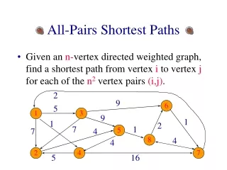
All-Pairs Shortest Paths. 15.1 最短路徑的特性. 最短路徑的結構: 所有最短路徑的子路徑均為最短路徑。 如 : (v i ,…,v k ,v j ) 為 v i 到 v j 的最短路徑,則 (v i ,…,v k ) 必為 v i 到 v k 的最短路徑。 即: δ(v i ,v j )=δ(v i ,v k )+w(v k ,v j ). 最短路徑的特性. 一個直覺的遞迴解: 定義 d (m) (i,j) 為包含至多 m 個邊自 i j 的最短路徑長度。則:. 利用遞迴解計算出最短路徑.

E N D
15.1 最短路徑的特性 • 最短路徑的結構:所有最短路徑的子路徑均為最短路徑。 • 如:(vi,…,vk,vj)為vi到vj的最短路徑,則(vi,…,vk)必為vi到vk的最短路徑。 • 即:δ(vi,vj)=δ(vi,vk)+w(vk,vj) All-Pairs Shortest Paths
最短路徑的特性 • 一個直覺的遞迴解:定義d(m)(i,j)為包含至多m個邊自ij的最短路徑長度。則: All-Pairs Shortest Paths
利用遞迴解計算出最短路徑 • 令n=|V|,如一圖無負迴圈,則d(n-1)(i,j)即為ij的最短路徑長度。 • 可以直覺使用動態規劃的方式來求出解,但耗時O(|V|3log|V|)反不如直接利用Dijkstra演算法直接求出所有點作為起點到其他點的最短路徑(以Linear array實做耗時O(|V|3))。 All-Pairs Shortest Paths
All-pairs Shortest Paths演算法 • 輸入: 一無負迴圈圖G=(V,E),|V|=n。n×n adjacency matrix W=(W[i,j]) All-Pairs Shortest Paths
All-pairs Shortest Paths演算法 • 輸出: n×n minimum distance matrix D=(D[i,j]) D[i,j]=δ(i,j)n×n predecessor matrix π=(π[i,j])若ij無路徑則π[i,j]=NIL, 否則π[i,j]紀錄ij最短路徑上j之前的點 π[i,j] i k j All-Pairs Shortest Paths
Extend-Shortest-Paths(D,W) { nrows[D] Let D’ = (D’[i,j]) be an nn matrix for i=1 to n do for j=1 to n do D’[i,j] for k=1 to n do D’[i,j]min(D’[i,j],D[i,k]+W[k,j]) return D’ } Time Complexity: O(n3) All-Pairs Shortest Paths
Slow-All-Pairs-Shortest-Paths(G,W) { n|V| D(1)W for m=2 to n-1 do D(m)Extend-Shortest-Paths(D(m-1),W) return D(n-1) } Time Complexity: O(n4) All-Pairs Shortest Paths
Faster-All-Pairs-Shortest-Paths(G,W) { n|V| D(1)=W m=1 while n-1>m do D(2m)Extend-Shortest-Paths(D(m),D(m)) m = 2m return D(m) } Time Complexity: O(n3logn) All-Pairs Shortest Paths
15.2 Floyd-Warshall演算法 • 主要利用不同的觀察找出新的遞迴式,使得演算法複雜度降低至O(n3),在邊數多的時候能有比Dijkstra演算法更迅速的求出所有的最短路徑。 • 若一ij的路徑為(i,u1,…,um,j),則我們稱u1,…,um為該路徑的Intermediate vertex(中間點)。 All-Pairs Shortest Paths
Floyd-Warshall演算法 • 假定點集合V={1,…,n},定義d(m)(i,j)為中間點僅可能為{1,…,m}最短的ij路徑長。故: All-Pairs Shortest Paths
Floyd-Warshall演算法正確性分析 • 考慮中間點僅可能為{1,…,k}。 • 如k不在ij最短路徑上,則中間點僅可能為{1,…,k-1},故此時:d(k)(i,j)=d(k-1)(i,j)。 All-Pairs Shortest Paths
Floyd-Warshall演算法正確性分析 • 如k在ij最短路徑上,則將ik及kj兩段分開看,這兩個路徑必然不可能有中間點為k,否則依照無負迴圈的假定,ik或kj不是最短路徑,違背最短路徑的性質。故此時:d(k)(i,j)=d(k-1)(i,k)+d(k-1)(k,j)。 中間點僅有{1,…,k-1} i k j 中間點僅有{1,…,k-1} All-Pairs Shortest Paths
Floyd-Warshall演算法 Floyd-Warshall(G,W) { n|V| D(0)W for k = 1 to n do for i = 1 to n do for j = 1 to n do if D(k-1)[i,j]>D(k-1)[i,k]+D(k-1)[k,j] then D(k)[i,j]D(k-1)[i,k]+D(k-1)[k,j] π[i,j] π[k,j] else D(k)[i,j]D(k-1)[i,j] return D(n) } Time Complexity: O(n3) All-Pairs Shortest Paths
建造Shortest path • 初始化π[i,j]時,如i=j或(i,j)∉E則初始為NIL,否則初始為i。 • 等執行完演算法後,則可利用Single-Source shortest path的方式,藉由Predecessor graph來建立出ij的最短路徑。 All-Pairs Shortest Paths
Floyd-Warshall範例 1 3 -4 8 7 5 2 6 2 4 1 4 3 -5 All-Pairs Shortest Paths
Floyd-Warshall範例 All-Pairs Shortest Paths
Floyd-Warshall範例 All-Pairs Shortest Paths
Floyd-Warshall範例 All-Pairs Shortest Paths
Floyd-Warshall範例 All-Pairs Shortest Paths
Floyd-Warshall範例 All-Pairs Shortest Paths
Floyd-Warshall範例 All-Pairs Shortest Paths
15.3 Johnson’s algorithm • Johnson’s演算法可用於計算All pairs shortest path問題。 • 在邊的數量不多的時候,如|E|=O(|V|log|V|)時,能有比Warshall-Floyd演算法較佳的效能。 • 其輸入需求是利用Adjacency list表示的圖。 All-Pairs Shortest Paths
Johnson’s algorithm • Johnson’s 演算法利用reweighing來除去負邊,使得該圖可以套用Dijkstra演算法,來達到較高的效能。 • Reweighing是將每個點v設定一個高度h(v),並且調整邊的weight function w(u,v)成為w’(u,v)=w(u,v)+h(u)-h(v)。 • 令δ‘(u,v)如此調整之後的最短距離,則原先的最短距離δ(u,v)=δ‘(u,v)-h(u)+h(v)。 All-Pairs Shortest Paths
Johnson’s algorithm Johnson(G) { compute G’, where V[G’]=V[G]{s} and E[G’]=E[G]{(s,v):vV[G] if Bellman-Ford(G’,w,s)=False then print “ a neg-weight cycle” elsefor each vertex v V[G’] set h(v)=(s,v) computed by Bellman-Ford algo. for each edge (u,v)E[G’] w’(u,v)=w(u,v)+h(u)-h(v) for each vertex u V[G] run Dijkstra(G,w’,u) to compute ’(u,v) for each v V[G] duv=’(u,v)-h(u)+h(v) return D } All-Pairs Shortest Paths
Johnson’s algorithm範例 4 3 7 8 -5 1 -4 2 6 All-Pairs Shortest Paths
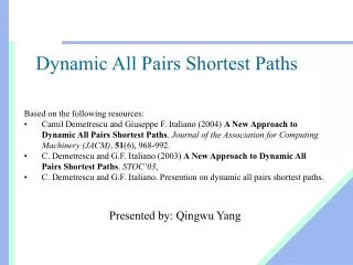
Johnson’s algorithm範例 0 0 加入一個點s,以及自s拉一條weight為0的邊到每一點。 4 3 7 0 8 s -5 1 -4 2 0 6 0 All-Pairs Shortest Paths
Johnson’s algorithm範例 0 -1 0 執行Bellman-Ford演算法,得到自s出發每一點的最短距離。 4 3 7 0 8 s 0 -5 -5 1 -4 2 0 -4 0 6 0 All-Pairs Shortest Paths
Johnson’s algorithm範例 -1 做完reweighting 0 4 10 13 0 -5 0 0 0 2 -4 0 2 All-Pairs Shortest Paths
Johnson’s algorithm範例 2/1 紅線部分是Shortest-paths tree。點的數字a/b代表自出發點(綠色點)出發,到達該點的最短路徑(Reweighting後的圖/原圖)。 0 4 10 13 0/0 2/-3 0 0 0 2 0/-4 2/0 2 All-Pairs Shortest Paths
Johnson’s algorithm範例 0/0 0 4 10 13 2/3 0/-4 0 0 0 2 2/-1 0/1 2 All-Pairs Shortest Paths
Johnson’s algorithm範例 0/4 0 4 10 13 2/7 0/0 0 0 0 2 2/3 0/5 2 All-Pairs Shortest Paths
Johnson’s algorithm範例 0/-1 0 4 10 13 2/2 0/-5 0 0 0 2 2/-2 0/0 2 All-Pairs Shortest Paths
Johnson’s algorithm範例 2/5 0 4 10 13 4/8 2/1 0 0 0 2 0/0 2/6 2 All-Pairs Shortest Paths
Johnson’s algorithm複雜度分析 • 執行一次Bellman-Ford。O(|V||E|)。 • 執行|V|次Dijkstra。 • 使用Fibonacci heap,總計O(|V|2log|V|+|V||E|) 。 • 使用Binary heap,總計O(|V||E|log|V|)。 • 當|E|足夠小,比Warshall-Floyd快。 All-Pairs Shortest Paths