Download
1 / 24
250 likes | 274 Vues
MECH 373 Instrumentation and Measurement. Lecture 2 (Course Website: Access from your “My Concordia” portal). Contents of today’s lecture: • Dealing with error – Error reduction techniques – Standards – Calibration. • Dynamic measurements

E N D
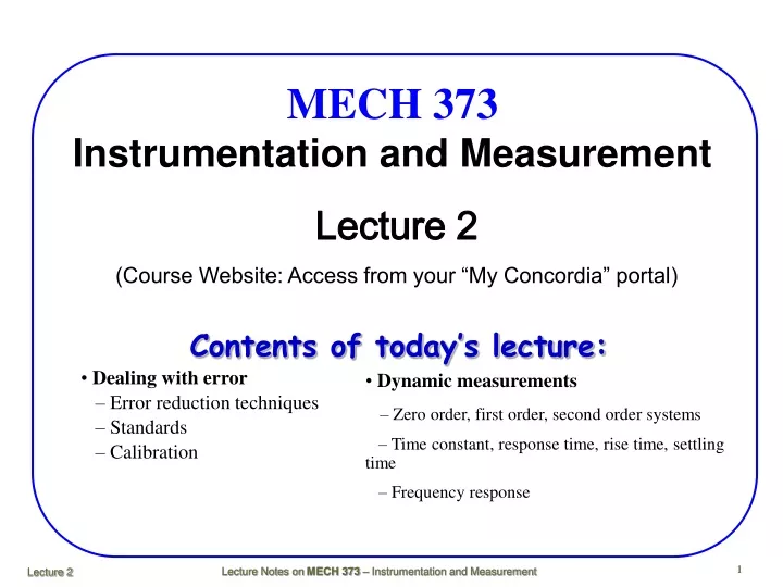
MECH 373Instrumentation and Measurement Lecture 2 (Course Website: Access from your “My Concordia” portal) Contents of today’s lecture: • Dealing with error – Error reduction techniques – Standards – Calibration • Dynamic measurements – Zero order, first order, second order systems – Time constant, response time, rise time, settling time – Frequency response 1
Output Input Measured valueof variables True valueof variables Essential Elements Measurement System SensingElement ConditioningElement ProcessingElement DisplayingElement 2
Sources of errors Improper sensing position Improper element calibration Improper data acquisition method Improper sampling rate Elements non-linearity Environment effects Types of Measurement Errors Characteristic of errors • Systematic errors • Random errors • Parameter tracking errors 4
Summary How to reduce the measurement errors? Topic in today’s lecture 5
Error Reduction Techniques (1) The mosteffectivemethodof reducingmeasurement error (systematic)is to: Set the sensing element at the right position. Area with low stress gradient and low temperature. 6
Error Reduction Techniques (2) An effectiveand useful methodof reducingmeasurement error (systematic)is to: Calibrate each element to eliminate or reduce bias. DC shift. Offset 7
Error Reduction Techniques (3) Anothereffectivemethodof reducingmeasurement error (systematic)is to: Setup a proper sampling rate for data acquisition. At least 2 times of the highest frequency of interest. D 8
Another effectivemethodof reducingmeasurement error (systematic and random)is to: compensate the environmental effects • Environmental effectsisolation: • Environmental inputcancellation: Error Reduction Techniques (4) 9
Random error reduction (5) Random errors – Originate from measuring systems and experimental systems. In measuring systems – Temperature effects on amplifier performance. Environmental causes – Electrical noise from electric and magnetic field around the equipments. Solution – Proper shielding or grounding the measuring systems – Minimise electrical noise. Statistical analysis – Large number of samples. 10
The first step before performing a measurement is instrument calibration When a measurement system is calibrated it is compared with some standard whose value is presumably known The standard may be a piece of equipment, an object having a well-defined physical attribute to be used as a comparison, or a well accepted technique known to produce a reliable value The accuracy of a standard needs to be higher than the one of the instrument being calibrated. A rule often followed is that the calibrated standard has an accuracy four times better than the instrument being calibrated Standards 12
The basic dimensions are: Mass - Kg Time - Second Length - meter Temperature – Celsius, Kelvin (0 K = -273.15C) and Fahrenheit Electric Current (Amp) ..... Basic Dimensions: Standards, Units 13
Relationship between measurement and true value is the first task performed in a measurement: calibration Calibration - Applying known input value (standard) to unknown measurement system for the purpose of observing the output and establishing an input-output relationship. Applying a range of known values for the input and observing the output – Develop a direct calibration curve. Use the calibration curve in later measurements to ascertain the unknown input value (actual value) based on the output value. Calibration 14
Calibration • Calibration: • A test in which known values of the input are applied to a measurement system (or sensor) for the purpose of observing the system (or sensor) output. • Static calibration: • A calibration procedure in which the values of the variable involved remain constant (do not change with time or change slowly) – static weights. • • Dynamic calibration: • When the variables of interest are time dependent and time-based information is need. The dynamic calibration determines the relationship between an input of known dynamic behavior and the measurement system output – Accelerometers. 15
In performing a static calibration, the following steps are necessary: Examine the construction of the instrument and identify and list all the possible inputs. Decide, as best as you can, which of the inputs will be significant in the application for which the instrument is to be calibrated – Establish range. Find an apparatus that will allow you to vary all the significant inputs over the ranges considered necessary. Find standards to measure inputs. By holding some inputs constant and varying others, record the output and develop the desired static input-output relation as a best-fit curve. Static Calibration 16
If the output data of a measurement system is to give a meaningful description of the measurement process, the data must form what is called a random sequence. In a calibration we specify that certain inputs must be held constant within certain limits. Those are the inputs that hopefully will have the most influence in the measurement. However, there are many extraneous input variables that are uncontrolled – environment effects. A reasonable assumption is that the aggregate of their effect on the instrument output will be of a random nature. We can then apply the least-squares method to find the best-fit curve – ‘Eye-ball’ approach. Best-fit Curve 17
Best-fit Line R = 1.290W – 0.374 18
Static calibration - Deviation Max. repeatability error – UP cycles 19
Static calibration - Average deviation Max. systematic error
Static calibration – Error summary Several cycles before data recording. Typical 5 cycles recommended for static calibration. ANSI/ISA(1979). Establish best fit curve (eye-ball). Output span: W = 0 lb., R = -0.374 lb. and W = 5 lb., R = 6.076 lb. O/S = 6.076 – (-0.374) = 6.45 lb. Accuracy limits – Max and min deviations from best fit line. +0.45 lb. at 0 lb. (down cycle), 7% of output span; -0.40 lb. at 2 lb (up cycle) - -6.2% of O/S.
Static calibration – Error summary Non-linearity – Average of all data taken for each weight value in both up and down cycles – Solid dots in Fig. E2.3(d). Max. = 0.41 lb. (6.4% of O/S) at 0 lb. Repeatability error – Max variability of successive measurements of same input value approached same loading direction – Fig. E2.3(c) At 1 lb. up cycle - Range -0.14 to -0.31 – 0.17 lb. 2.6% of O/S, +/-1.3% of output span.
Max hysteresis error – Max difference between the Up and the correspond Down reading for any calibration cycle – Table E2.3(b). – Cycle 3 at 2.5 lb., -0.39 lb. in up cycle, -0.13 lb., in down cycle. Total = 0.52 lb., 8.1% of O/S, +/-4.05% of O/S. Static calibration – Error summary
Max. systematic error – Max deviation of the averaged calibrated values (average of up and down readings) for all cycles – Fig. E3.2(d). At 0 lb., +0.41lb, +6.4% of O/S. At 2.5 lb., -0.35lb, -5.4% of O/S. Max. random error – repeatability error – same input and same loading direction. At 1 lb. in up cycles, Cycle 3 = -0.14 lb., Cycle 5 = -0.31 lb. Range = 0.17 lb, 2.6% of O/S, +/- 1.3% of O/S. Static calibration – Error summary