Download
1 / 55
560 likes | 585 Vues
Explore the history, goals, and hardware of neural networks. Learn about cortical neurons, synapses, brain functionality, and idealized neuron models. Discover the eras of neural computation and adaptability in the brain.

E N D
CSC2535: Computation in Neural NetworksLecture 1: The history of neural networks Geoffrey Hinton All lecture slides are available as .ppt, .ps, & .htm at www.cs.toronto.edu/~hinton
Why study neural computation? • The motivation is that the brain can do amazing computations that we do not know how to do with a conventional computer. • Vision, language understanding, learning ….. • It does them by using huge networks of slow neurons each of which is connected to thousands of other neurons. • Its not at all like a conventional computer that has a big, passive memory and a very fast central processor that can only do one simple operation at a time. • It learns to do these computations without any explicit programming.
The goals of neural computation • To understand how the brain actually works • Its big and very complicated and made of yukky stuff that dies when you poke it around • To understand a new style of computation • Inspired by neurons and their adaptive connections • Very different style from sequential computation • should be good for things that brains are good at (e.g. vision) • Should be bad for things that brains are bad at (e.g. 23 x 71) • To solve practical problems by using novel learning algorithms • Learning algorithms can be very useful even if they have nothing to do with how the brain works
Overview of this lecture • Brief description of the hardware of the brain • Some simple, idealized models of single neurons. • Two simple learning algorithms for single neurons. • The perceptron era (1960’s) • What they were and why they failed. • The associative memory era (1970’s) • From linear associators to Hopfield nets. • The backpropagation era (1980’s) • The backpropagation algorithm
A typical cortical neuron • Gross physical structure: • There is one axon that branches • There is a dendritic tree that collects input from other neurons • Axons typically contact dendritic trees at synapses • A spike of activity in the axon causes charge to be injected into the post-synaptic neuron • Spike generation: • There is an axon hillock that generates outgoing spikes whenever enough charge has flowed in at synapses to depolarize the cell membrane axon body dendritic tree
Synapses • When a spike travels along an axon and arrives at a synapse it causes vesicles of transmitter chemical to be released • There are several kinds of transmitter • The transmitter molecules diffuse across the synaptic cleft and bind to receptor molecules in the membrane of the post-synaptic neuron thus changing their shape. • This opens up holes that allow specific ions in or out. • The effectiveness of the synapse can be changed • vary the number of vesicles of transmitter • vary the number of receptor molecules. • Synapses are slow, but they have advantages over RAM • Very small • They adapt using locally available signals (but how?)
How the brain works • Each neuron receives inputs from other neurons • Some neurons also connect to receptors • Cortical neurons use spikes to communicate • The timing of spikes is important • The effect of each input line on the neuron is controlled by a synaptic weight • The weights can be positive or negative • The synaptic weights adapt so that the whole network learns to perform useful computations • Recognizing objects, understanding language, making plans, controlling the body • You have about 10 neurons each with about 10 weights • A huge number of weights can affect the computation in a very short time. Much better bandwidth than pentium. 11 3
Modularity and the brain • Different bits of the cortex do different things. • Local damage to the brain has specific effects • Adult dyslexia; neglect; Wernicke versus Broca • Specific tasks increase the blood flow to specific regions. • But cortex looks pretty much the same all over. • Early brain damage makes functions relocate • Cortex is made of general purpose stuff that has the ability to turn into special purpose hardware in response to experience. • This gives rapid parallel computation plus flexibility • Conventional computers get flexibility by having stored programs, but this requires very fast central processors to perform large computations.
Idealized neurons • To model things we have to idealize them (e.g. atoms) • Idealization removes complicated details that are not essential for understanding the main principles • Allows us to apply mathematics and to make analogies to other, familiar systems. • Once we understand the basic principles, its easy to add complexity to make the model more faithful • It is often worth understanding models that are known to be wrong (but we mustn’t forget that they are wrong!) • E.g. neurons that communicate real values rather than discrete spikes of activity.
Linear neurons • These are simple but computationally limited • If we can make them learn we may get insight into more complicated neurons bias th i input y 0 weight on b 0 output th input i index over input connections
Binary threshold neurons • McCulloch-Pitts (1943): influenced Von Neumann! • First compute a weighted sum of the inputs from other neurons • Then send out a fixed size spike of activity if the weighted sum exceeds a threshold. • Maybe each spike is like the truth value of a proposition and each neuron combines truth values to compute the truth value of another proposition! 1 1 if y 0 0 otherwise z threshold
Linear threshold neurons These have a confusing name. They compute a linear weighted sum of their inputs The output is a non-linear function of the total input y 0 otherwise 0 z threshold
Sigmoid neurons • These give a real-valued output that is a smooth and bounded function of their total input. • Typically they use the logistic function • They have nice derivatives which make learning easy (see lecture 4). • If we treat as a probability of producing a spike, we get stochastic binary neurons. 1 0.5 0 0
Feedforward networks These compute a series of transformations Typically, the first layer is the input and the last layer is the output. Recurrent networks These have directed cycles in their connection graph. They can have complicated dynamics. More biologically realistic. Types ofconnectivity output units hidden units input units
Types of learning task • Supervised learning • Learn to predict output when given input vector • Who provides the correct answer? • Reinforcement learning • Learn action to maximize payoff • Not much information in a payoff signal • Payoff is often delayed • Unsupervised learning • Create an internal representation of the input e.g. form clusters; extract features • How do we know if a representation is good?
The neuron has a real-valued output which is a weighted sum of its inputs The aim of learning is to minimize the discrepancy between the desired output and the actual output How do we measure the discrepancies? Do we update the weights after every training case? Why don’t we solve it analytically? A learning algorithm for linear neurons weight vector input vector Neuron’s estimate of the desired output
The delta rule • Define the error as the squared residuals summed over all training cases, n • Now differentiate to get error derivatives for the weight on the connection coming from input, i • The batch delta rule changes the weights in proportion to their error derivatives summed over all training cases
The error surface • The error surface lies in a space with a horizontal axis for each weight and one vertical axis for the error. • It is a quadratic bowl. • Vertical cross-sections are parabolas. • Horizontal cross-sections are ellipses. w1 E w2
Batch learning does steepest descent on the error surface Online learning zig-zags around the direction of steepest descent Online versus batch learning constraint from training case 1 w1 w1 constraint from training case 2 w2 w2
The direction of steepest descent does not point at the minimum unless the ellipse is a circle. The gradient is big in the direction in which we only want to travel a small distance. The gradient is small in the direction in which we want to travel a large distance. This equation is sick. The RHS needs to be multiplied by a term of dimension w^2. Alater lecture will cover ways of fixing this problem. Convergence speed
Adding biases • A linear neuron is a more flexible model if we include a bias. • We can avoid having to figure out a separate learning rule for the bias by using a trick: • A bias is exactly equivalent to a weight on an extra input line that always has an activity of 1.
The combination of an efficient learning rule for binary threshold neurons with a particular architecture for doing pattern recognition looked very promising. There were some early successes and a lot of wishful thinking. Some researchers were not aware of how good learning systems are at cheating. The perceptron era (the 1960’s) 1 y 0 z threshold 1 if 0 otherwise
The perceptron convergence procedure: Training binary threshold neurons as classifiers • Add an extra component with value 1 to each input vector. The “bias” weight on this component is minus the threshold. Now we can forget the threshold. • Pick training cases using any policy that ensures that every training case will keep getting picked • If the output is correct, leave its weights alone. • If the output is 0 but should be 1, add the input vector to the weight vector. • If the output is 1 but should be 0, subtract the input vector from the weight vector • This is guaranteed to find a suitable set of weights if any such set exists. • There is no need to choose a learning rate.
Imagine a space in which each axis corresponds to a weight. A point in this space is a weight vector. Each training case defines a plane. On one side of the plane the output is wrong. To get all training cases right we need to find a point on the right side of all the planes. Weight space an input vector with correct answer=0 wrong right bad weights good weights right wrong an input vector with correct answer=1 o the origin
Consider the squared distance between any satisfactory weight vector and the current weight vector. Every time the perceptron makes a mistake, the learning algorithm moves the current weight vector towards all satisfactory weight vectors (unless it crosses the constraint plane). So consider “generously satisfactory” weight vectors that lie within the feasible region by a margin at least as great as the largest update. Every time the perceptron makes a mistake, the squared distance to all of these weight vectors is always decreased by at least the squared length of the smallest update vector. Why the learning procedure works margin right wrong
What binary threshold neurons cannot do Data Space (not weight space) • A binary threshold output unit cannot even tell if two single bit numbers are the same! Same: (1,1) 1; (0,0) 1 Different: (1,0) 0; (0,1) 0 • The four input-output pairs give four inequalities that are impossible to satisfy: 0,1 1,1 weight plane output =1 output =0 1,0 0,0 The positive and negative cases cannot be separated by a plane
The standard perceptron architecture The input is recoded using hand-picked features that do not adapt. These features are chosen to ensure that the classes are linearly separable. Only the last layer of weights is learned. The output units are binary threshold neurons and are learned independently. output units non-adaptive hand-coded features input units This architecture is like a generalized linear model, but for classification instead of regression.
Is preprocessing cheating? • It seems like cheating if the aim to show how powerful learning is. The really hard bit is done by the preprocessing. • Its not cheating if we learn the non-linear preprocessing. • This makes learning much more difficult and much more interesting.. • Its not cheating if we use a very big set of non-linear features that is task-independent. • Support Vector Machines make it possible to use a huge number of features without much computation or data.
What can perceptrons do? • They can only solve tasks if the hand-coded features convert the original task into a linearly separable one. • How difficult is this? • In the 1960’s, computational complexity theory was in its infancy. Minsky and Papert (1969) did very nice work on the spatial complexity of making a task linearly separable. They showed that: • Some tasks require huge numbers of features • Some tasks require features that look at all the inputs. • They used this work to correctly discredit some of the exaggerated claims made for perceptrons. • But they also used their work in a major ideological attack on the whole idea of statistical pattern recognition. • This had a huge negative impact on machine learning which took about 15 years to recover from its rejection of statistics.
Some of Minsky and Papert’s claims • Making the features themselves be adaptive or adding more layers of features won’t help. • Graphs with discretely labeled edges are a much more powerful representation than feature vectors. • Many AI researchers claimed that real numbers were bad and probabilities were even worse. • We should not try to learn things until we have a proper understanding of how to represent them • The “black box” approach to learning is deeply wrong and indicates a deplorable failure to comprehend the power of good new-fashioned AI. • The funding that ARPA was giving to statistical pattern recognition should go to good new-fashioned Artificial Intelligence at MIT. • At the same time as this attack, NSA was funding secret work on learning hidden Markov models which turned out to be much better than heuristic AI methods at recognizing speech.
There is a simple solution that requires N hidden units that see all the inputs Each hidden unit computes whether more than M of the inputs are on. This is a linearly separable problem. There are many variants of this solution. It can be learned by backpropagation and it generalizes well if: The N-bit even parity task +1 output -2 +2 -2 +2 >0 >1 >2 >3 1 0 1 0 input
Even for simple line drawings, we need exponentially many features. Removing one segment can break connectedness But this depends on the precise arrangement of the other pieces. Unlike parity, there are no simple summaries of the other pieces that tell us what will happen. Connectedness is easy to compute with an iterative algorithm. Start anywhere in the ink Propagate a marker See if all the ink gets marked. Connectedness is hard to compute with a perceptron
What kind of features are required to distinguish two different patterns of 5 pixels independent of position and orientation? Do we need to replicate T and C templates across all positions and orientations? Looking at pairs of pixels will not work Looking at triples will work if we assume that each input image only contains one object. Distinguishing T from C in any orientation and position Replicate the following two feature detectors in all positions + - - + + + If any of these equal their threshold of 2, it’s a C. If not, it’s a T.
The associative memory era (the 1970’s) • AI researchers persuaded people to abandon perceptrons and much of the research stopped for a decade. • During this “neural net winter” a few researchers tried to make associative memories out of neural networks. The motivating idea was that memories were cooperative patterns of activity over many neurons rather than activations of single neurons. Several models were developed: • Linear associative memories • Willshaw nets (binary associative memories) • Binary associative memories with hidden units • Hopfield nets
It is shown pairs of input and output vectors. It modifies the weights each time it is shown a pair. After one sweep through the training set it must “retrieve” the correct output vector for a given input vector We are not asking it to generalize Linear associative memories input vector output vector
If the input vector consists of activation of a single unit, all we need to do is set the weight at each synapse to be the product of the pre- and post-synaptic activities This is the Hebb rule. If the input vectors form an orthonormal set, the same Hebb rule works because we have merely applied a rotation to the “localist” input vectors. But we can now claim that we are using distributed patterns of activity as representations. Boring! Trivial linear associative memories 0 0 1 0 0 input vector output vector
These use binary activities and binary weights. They can achieve high efficiency by using sparse vectors . Turn on a synapse when input and output units are both active. For retrieval, set the output threshold equal to the number of active input units This makes false positives improbable Willshaw nets 1 0 1 0 0 in 0 1 0 0 1 output units with dynamic thresholds
Hopfield Nets • A Hopfield net is composed of binary threshold units with recurrent connections between them. Recurrent networks of non-linear units are generally very hard to analyze. They can behave in many different ways: • Settle to a stable state • Oscillate • Follow chaotic trajectories that cannot be predicted far into the future. • But Hopfield realized that if the connections are symmetric, there is a global energy function • Each “configuration” of the network has an energy. • The binary threshold decision rule causes the network to settle to an energy minimum.
The energy function • The global energy is the sum of many contributions. Each contribution depends on one connection weight and the binary states of two neurons: • The simple quadratic energy function makes it easy to compute how the state of one neuron affects the global energy:
Pick the units one at a time and flip their states if it reduces the global energy. Find the minima in this net If units make simultaneous decisions the energy could go up. Settling to an energy minimum -4 3 2 3 3 -1 -1 -100 0 0 +5 +5
How to make use of this type of computation • Hopfield proposed that memories could be energy minima of a neural net. • The binary threshold decision rule can then be used to “clean up” incomplete or corrupted memories. • This gives a content-addressable memory in which an item can be accessed by just knowing part of its content (like google) • It is robust against hardware damage.
Storing memories • If we use activities of 1 and -1, we can store a state vector by incrementing the weight between any two units by the product of their activities. • Treat biases as weights from a permanently on unit • With states of 0 and 1 the rule is slightly more complicated.
Spurious minima • Each time we memorize a configuration, we hope to create a new energy minimum. But what if two nearby minima merge to create a minimum at an intermediate location? This limits the capacity of a Hopfield net. • Using Hopfield’s storage rule the capacity of a totally connected net with N units is only 0.15N memories. • This does not make efficient use of the bits required to store the weights in the network. • Willshaw nets were much more efficient!
Avoiding spurious minima by unlearning • Hopfield, Feinstein and Palmer suggested the following strategy: • Let the net settle from a random initial state and then do unlearning. • This will get rid of deep , spurious minima and increase memory capacity. • Crick and Mitchison proposed unlearning as a model of what dreams are for. • That’s why you don’t remember them (Unless you wake up during the dream) • But how much unlearning should we do? • And can we analyze what unlearning achieves?
Boltzmann machines: Probabilistic Hopfield nets with hidden units • If we add extra units to a Hopfield net that are not part of the input or output, and we also make the neurons stochastic, lots of good things happen. • Instead of just settling to the nearest energy minimum, the stochastic net can jump over energy barriers. • This allows it to find much better minima, which is very useful if we are doing non-linear optimization. • With enough hidden units the net can create energy minima wherever it wants to (e.g. 111, 100, 010, 001). A Hopfield net cannot do this. • There is a simple local rule for training the hidden units. This provides a way to learn features, thus overcoming the fundamental limitation of perceptron learning. • Boltzmann machines are complicated. They will be described later in the course. They were the beginning of a new era in which neural networks learned features, instead of just learning how to weight hand-coded features in order to make a decision.
The backpropagation era: (1980’s & early 90’s) • Networks without hidden units are very limited in the input-output mappings they can model. • More layers of linear units do not help. Its still linear. • Fixed output non-linearities are not enough • We need multiple layers of adaptive non-linear hidden units. This gives us a universal approximator. But how can we train such nets? • We need an efficient way of adapting all the weights, not just the last layer. This is hard. Learning the weights going into hidden units is equivalent to learning features. • Nobody is telling us directly what hidden units should do.
Learning by perturbing weights • Randomly perturb one weight and see if it improves performance. If so, save the change. • Very inefficient. We need to do multiple forward passes on a representative set of training data just to change one weight. • Towards the end of learning, large weight perturbations will nearly always make things worse. • We could randomly perturb all the weights in parallel and correlate the performance gain with the weight changes. • Not any better because we need lots of trials to “see” the effect of changing one weight through the noise created by all the others. output units hidden units input units Learning the hidden to output weights is easy. Learning the input to hidden weights is hard.
The idea behind backpropagation • We don’t know what the hidden units ought to do, but we can compute how fast the error changes as we change a hidden activity. • Instead of using desired activities to train the hidden units, use error derivatives w.r.t. hidden activities. • Each hidden activity can affect many output units and can therefore have many separate effects on the error. These effects must be combined. • We can compute error derivatives for all the hidden units efficiently. • Once we have the error derivatives for the hidden activities, its easy to get the error derivatives for the weights going into a hidden unit.
A change of notation • For simple networks we use the notation x for activities of input units y for activities of output units z for the summed input to an output unit • For networks with multiple hidden layers: y is used for the output of a unit in any layer x is the summed input to a unit in any layer The index indicates which layer a unit is in.
Non-linear neurons with smooth derivatives • For backpropagation, we need neurons that have well-behaved derivatives. • Typically they use the logistic function • The output is a smooth function of the inputs and the weights. 1 0.5 0 Its odd to express it in terms of y. 0