Download

1 / 160
1.6k likes | 1.6k Vues
Learn about the principles of Principal Component Analysis (PCA) and various data visualization techniques for effective data analysis. Topics covered include scaling of variables, correlation PCA, transformations, automatic log transformations, and heat map views.

E N D
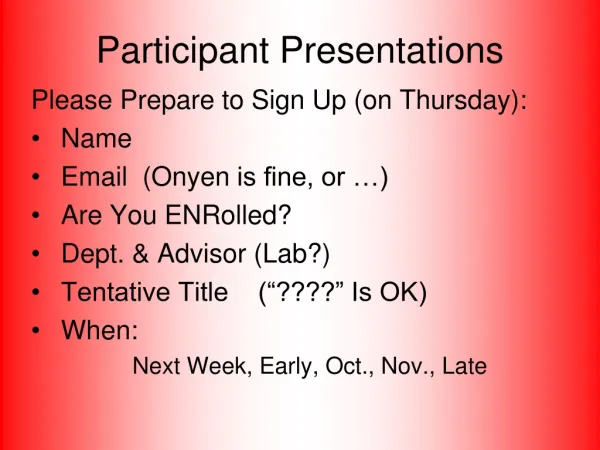
Participant Presentations Starting This Thursday: 11: 35 Benjamin Leinwand 11:40 Keerthi Anand Notes: • Can Use USB Device • Or Remote Log-In, Set Up Before Class • Have Title Page With: • Your Name • Your Affiliation Check Website For Schedule
Limitation of PCA Strongly Feels Scaling of Each Variable Consequence: May want to standardize each variable (i.e. subtract , divide by ) Also called Whitening Equivalent Approach: Base PCA on Correlation Matrix Called Correlation PCA
Correlation PCA Toy Example Contrasting Cov. vs. Corr. 1st Comp: Nearly Flat 2nd Comp: Contrast 3rd & 4th: Look Very SmallSince CommonAxes
Correlation PCA Toy Example Contrasting Cov. vs. Corr. Correlation “Whitened” Version All Much Different Which Is “Right” ???
Transformations Recall Log for Mortality and RNAseq Data • Useful Method for Data Analysis • Apply to Marginal Distributions (i.e. to Individual Variables) • Idea: Put Data on Right Scale • Common Example: • Data Orders of Magnitude Different • Log10 Puts Data on More Analyzable Scale
Transformations Box – Cox Transformations Why this strange form? Instead of just Reason: Nicer Behavior as , Try It Out Using L’Hopital’s Rule
Transformations Few Large Values Can Dominate Analysis
Transformations Log Scale Gives All More Appropriate Weight Note: Orders Of Magnitude Log10 most Interpretable
Automatic Transformations Family of transformation functions Comments • Single family for both positive and negative skewness • Parameter value selection is independent of data magnitude • As : transformation + standardization standardization only
Automatic Transformations Standardization • Subtract median (robust center) • Divide by of the MAD (robust scale) (Mean Absolute Deviation from the median) Winsorization • Threshold based on extreme value theory (see Feng et al (2016) for details)
Melanoma Data Much Nicer Distributions
Revisit Gene Expression Add In Automatic Log Transformed PCA Ovarian (o) & Uterine (+) Cancer Cases Proj’ns on Mean Difference Dir’n Note Much Better
Revisit Gene Expression ROC Curve Much Better For Log Transformations
Data Visualization Overview of Visualization Methods: • Curve Views (FDA) • Scatterplot Matrices (Shows Relationships) • Marginal Distributions • Heat-Map Views
Heat-Map Views Main Idea: • Look at Full Data Matrix • As an Image (Rectangular Array of “Pixels”) • Coding Values with Colors (Gray Levels)
Heat-Map Views Actually Gray Level Is Also Good For: “No Pivotal Value (e.g. 0) To HighLight” Some Principles: For Nonnegative Data (i. e. all ) Gray Level is Informative (& Not Distracting) Some Advocate a RAINBOW Gives “Greater Range”??? Borland & Taylor (2007) Disagree Over Perceptual Interpretation (What Is Equally Spaced ???)
Heat-Map Views Some Principles: Ordering Rows and Columns Really Matters Clustering Columns Highlights Relationships Clustering “Knobs”: Hierarchical with Euclidean Distance & Average Linkage
Heat-Map Views Population Structure Invisible w/ Random Order Some Principles: Ordering Rows and Columns Really Matters Clustering Columns & Rows is Crucial
Heat-Map Views Dist’n of Values, with Usual Jitter Plot + Smooth Histo Some Principles: Color Scale is Also Critical Equal Bin Spacing Toy Example Many Small Values & Few Large Ones Results in Very Poor Contrast
Heat-Map Views Natural Approach (to Skewed Dist’n): Log Transformation Same Toy Example Much Better Scaling, Using More of the Color Range Much Better Contrast, Now See 4 Peaks
Heat-Map Views Natural Approach (to Skewed Dist’n): Quantile Scaling (= #s in Each Bin) Same Toy Example Non-Equally Spaced Bins Can Look at Either OriginalOr Log View Good or Bad? Peaks Less Prominent Far More Contrast
Heat-Map Views “Best” Choice of Color Scaling: Context Dependent • Equally Spaced (Most Interpretable?) • Log Spacing (Can Be Very Useful) • Quantile Spacing (Also Useful) Should Look At Several & Decide
Heat-Map Views Important Color Scale Choice: Endpoints of Color Range Note Ending Color Used Beyond Range Color Cutoffs? When No Pivotal Value (e.g. 0 Not Important) Recommend Quantiles, e.g. & Often Worth Twiddling These
Heat-Map Views Color Choice When 0 Needs Highlighting A Recommendation ( Many): Important: Middle White Highlights 0 Shade Indicates Magnitude Red for <0? (Econ.) for >0? (Climatology)
Heat-Map Views Color Choice When 0 Needs Highlighting A Recommendation ( Many): Why Not Red-Green??? (Common in Bioinf.) ~10% of European (Ancestry) Males are Red-GreenColorblind Most Other Choices as Good as This
Heat-Map Views Caution: Many Packages Do This! Color Choice When 0 Needs Highlighting Endpoints? ( & Will Re-Center!) Recommend Using Absolute Quantiles: Where is -th Quantile of
Heat-Map Views Larger Example: , Major Issue: Most Computer Displays Have Only a Few Thousand Pixels of Resolution So Cannot See Full Matrix Most Displays Compensate With Ad Hoc Rules Designed for Text and Natural Images Can Miss Important Aspects of the Data
Will See OK For This Data Heat-Map Views Larger Example: , Simple Approach Here: Study 1st Rows Looks Totally Random? Have Done Both Column And Row Clustering
Heat-Map Views Conclude: Heat Map Worse Than Scatterplot In This Case Larger Example: , Revisit With Scatterplot Matrix View Colored 1st 100 & 2nd 100 Clear Cluster Structure Hidden by Noise in Heatmap View! Is This Real (or Artifact)? &
Heat-Map Views For Opposite Answer Consider Another Data Set () with Curve View: Very Noisy 1st 25 Features >> 2nd 25 Two Clear Clusters Understand Pop’n Structure???
Heat-Map Views Data Source is Above Example: Gives Quicker Impression of Structure More Natural View Than Curves 2 Clusters 1st Features Larger
Heat-Map Views One More Point (From This Example): Than Both Separated Mean +/- Curves Easier to Understand
Heat-Map Views Which Data View Is “Best”??? • Heat Maps? • Curves? • Scatterplots?
Heat-Map Views Which Data View Is “Best”??? Simon Sheather Quote: “Every Dog Has His Day”
Heat-Map Views “Every Dog Has His Day” Idea: Any Data Analytic Method Somebody Likes Has Some Situations Where It Is “Best” & Of Course Others Where It Is Poor (Will See This Again)
Heat-Map Views Some Overview Papers: History: Wilkinson & Friendly (2009) Criticism of Common Color Choices: Borland & Taylor (2007)
Scatterplot Views All Based on Projections Now Consider Other Directions Beyond PCA
Scatterplot Views Summarize Other Directions to Project On • Classification Directions (e.g. DWD) • Independent Component Analysis • Fourier Basis Directions • Wavelet Basis Directions • Nonnegative Matrix Factorization Might Discuss Later
Scatterplot Views Summarize Other Directions to Project On • Known Modes of Variation Izem & Kingsolver (2007), Izem & Marron (2007) • Maximal Smoothness Directions Gaydos et. al (2013), Kingsolver et. al (2015), Zhang et al. (2014) • Maximal Data Piling (Will Explore Later)
Distance Methods Main Idea: Approach to Data Lying in Complicated Space (PCA Makes No Sense In Nonlinear Spaces) However, Often Have Notion of “Distance” I.e. Metric on Metric Space So Base Analysis on Distances
Distance Methods Given a metric on the Object Space And Data Objects Define Distance Matrix:
Distance Methods Common Choices of Metric (on ): Classical & Corresponds to Intuition Very Good at Downweighting Outliers Think Polar Coordinates, Focus on Angular Component and Ignore Radii
Distance Methods Major Consumers of Based Analyses Early Machine Learning Call Related Analyses “Kernel Trick” (Discuss More Later)
Distance Methods Notions of Sample Centerpoint? Conventional Sample Mean in : Note: Uses Linear Operations, Not Available in General
Distance Methods Approach: Replace Linear Op’s with Optimization Fréchet (1948) Mean: Start With Candidate Point Move Around to Min Sum of SquaredDist’s
Distance Methods Why Squared Distance? In , Using Metric , Can Show FréchetMean = I. e. Fréchet Mean is Generalization of Sample Mean
Distance Methods FréchetSample Mean, Toy Example Start With Candidate Point Move Around to Min Sum of Squared Dist’s
Distance Methods FréchetSample Mean, Toy Example Recall “Center Of Mass” Interpretretation Note: Outlier Pulls Mean Out of Convex Hull Of Other 4 Points Known Problem with Mean: Not Robust Against Outliers Min Looks Like Sample Mean???
Distance Methods Robust Variation: Fréchet (1948) Median: Again Start With Candidate Point Move Around to Min Sum of Distances
Distance Methods FréchetSample Median, Toy Example Better Robustness! Start With Candidate Point Move Around to Min Sum of Squared Dist’s