Mathematical models for mass and heat transport in porous media

1. Mathematical models for mass and heat transport in porous media Stefan Balint and Agneta M.Balint West University of Timisoara, RomaniaFaculty of Mathematics- Computer ScienceFaculty of Physics balint@balint.uvt.ro; balint@physics.uvt.ro Summer University, Vrnjacka Banja, October 2007

2. The presentation is focused on the mathematical modeling of mass and heat transport processes in porous media. • Basic concepts as porous media, mathematical models and the role of the model in the investigation of the real phenomena are discussed. • Several mathematical models as ground water flow, diffusion, adsorption, advection, macrotransport in porous media are presented and the results with respect to available experimental information are compared. Summer University, Vrnjacka Banja, October 2007

3. TOPICS: • MATHEMATICAL MODELING • POROUS MEDIA • FLUID FLOW IN A POROUS MEDIA • GROUNDWATER FLOW • MASS TRANSPORT IN POROUS MEDIA • COMPUTATIONAL RESULTS TESTED AGAINST EXPERIMENTAL RESULTS • HEAT TRANSPORT IN POROUS MEDIA • COMPUTED CONDUCTIVITY FOR THE HEAT TRANSPORT IN POROUS MEDIA TESTED AGAINST EXPERIMENTAL RESULTS Summer University, Vrnjacka Banja, October 2007

4. 1.MATHEMATICAL MODELING • Mathematical modeling is a concept that is difficult to define. It is first of all applied mathematics or more precisely, in physics applied mathematics. • According to A.C. Fowler: Mathematical Models in the Applied Sciences, Cambridge University Press, 1998 : • “Since there are no rules, and an understanding of the “right” way to model there are few texts that approach the subject in a serious way, one learns to model by practice, by familiarity with a wealth of examples.” Summer University, Vrnjacka Banja, October 2007

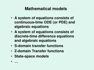
5. Applied mathematicians have a procedure, almost a philosophy that they apply when building models. • First, there is a phenomenon of interest that one wants to describe and to explain. Observations of the phenomenon lead, sometimes after a great deal of effort, to a hypothetical mechanism that can explain the phenomenon. The purpose of a mathematical model has to be to give a quantitative description of the mechanism. • Usually the quantitative description is made in terms of a certain number of variables (called the model variables) and the mathematical model isa set ofequations concerning the variables. • In formulating continuous models, there are three main ways of presenting equations for the model variables. • The classical procedure is to formulate exact conservation laws. The laws of mass, momentum and energy conservation in fluid mechanics are obvious examples of these. • The second procedure is to formulate constitutive relations between variables, which may be based on experiment or empirical reasoning (Hook law). • The third procedure is to use “hypothetical laws” based on quantitative reasoning in the absence of precise rules (Lotka-Volterra law). . Summer University, Vrnjacka Banja, October 2007

6. The analysis of a mathematical model leads to results that can be tested against the observations. • The model also leads to predictions which, if verified, lend authenticity to the model • It is important to realize thatall models are idealizations and are limited in their applicability. In fact, one usually aims to over-simplify; the idea is that if the model is basically right, then it can subsequently be made more complicated, but the analysis of it is facilitated by having treated a simpler version first. Summer University, Vrnjacka Banja, October 2007

7. 2. POROUS MEDIA • Example 1. The soil • Soil consists of an aggregation of variously sized mineral particles (MP) and the “pore spaces” (PS) between the particles. ( MP –green, PS – red) Figure 1. • When the “pore space” is completely full of water, then the soil is saturated. • When the “pore space” contains both water and air, then the soil isunsaturated. • In exceptional circumstances, soil can become desiccated. But, usually there is some water present. Summer University, Vrnjacka Banja, October 2007

8. Exemple 2.The column of the length 2m, filled with a quasi uniform quartz sand, of mean diameter 1.425 mm used by Bues and Aachib in the experiment reported in “Influence of the heterogeneity of the solutions on the parameters of miscible displacements in saturated porous medium, Experiments in fluids”, 11, Springer Verlag, 25-32, (1991). is a porous media. • Definition 1.A porous media is an array of a great number of variously sized fixed solid particles possessing the property that the volume concentration of solids is not small. (Soil). • Often it is characterized by its porosity Φ (i.e. the pore volume fraction) and its grain sized. The latter characterizes the “coarseness” of the medium. • Definition 2.A periodic porous media is a porous media having the property that the fixed solid particles are identical and the whole media is a periodic system of cells which are replicas of a standard (representative) cell (experimental column). Summer University, Vrnjacka Banja, October 2007

9. Figure 2. Periodic porous media Summer University, Vrnjacka Banja, October 2007

10. 3. FLUID FLOW IN A POROUS MEDIA • An incompressible viscous fluid moves in the “pore space” of a porous media, according to the Navier-Stokes equations: • (3.1) • satisfying the incompressibility condition: • (3.2) • where: is the fluid flow velocity; p is the pressure, ρ is the fluid density, μ is the fluid viscosity and is the density of the volume force acting in the fluid. • It is important to realize, that eqs. (3.1), (3.2) are valid only in the “pore space” (x belongs to the “pore space”). They can be obtained from the mass and momentum conservation laws and constitutive relations characterizing viscous fluids. Summer University, Vrnjacka Banja, October 2007

11. On the boundary of the fixed solid particles the fluid flow velocity has to satisfy the non slip condition: • (3.3) • Unfortunately, the boundary value problem (3.1), (3.2), (3.3) even in the case of a very slow stationary flow (Stokes flow), can not be solved numerically in a real situation due to the great number of the boundaries of fixed solid particles. • Consequently, the mathematical model defined by the eqs. (3.1), (3.2), (3.3) can not be analyzed numerically in a real case and can not be tested against the observations. • Several models for flow through porous media are based on a periodic array of spheres. • Hasimoto H. in On the periodic fundamental solution of the Stokes equations and their application to viscous flow passed a cubic array of spheres”, J.Fluid Mech.,5, 317-328 (1959). obtained the periodic fundamental solution to the Stokes problem by Fourier series expansion, and applied the results analytically to a dilute array of uniform spheres. • Sangani A.S., Acrivos A. in “Slow flow through a periodic array of spheres”, Int.J. Multiphase Flow, 8(4), 343-360 (1982) extended the approximation of Hasimoto to calculate the drag force for higher concentration. Summer University, Vrnjacka Banja, October 2007

12. - Zick A.A. and Homsy G.M. in “Stokes flow through periodic arrays of spheres”, J.FluidMech.,115, 13-26 (1982).use Hasimoto’s fundamental solution to formulate an integral equation for the force distribution on an array of spheres for arbitrary concentration. By numerical solution of the integral equation, results for packed spheres were obtained, for several porosity values. • - Continuous variation of porosity was examined only when the particles are in suspension. • - Strictly numerical computations have been made earlier, based on series of trial functions and the Galerkin method, for cubic packing of spheres in contact : • Snyder L.J. and Stewart W.A. “Velocity and pressure profiles for Newtonian creeping flow in regularpacked beds of spheres”, A.I.Ch.J.,12(1), 167-173 (1966). • Sorensen J.P. and Stewart W.E. “Computation of forced convection in slow flow through ducts and packed beds. II. Velocity profile in a simple cubic array of spheres, Chem.Engng.Sci., 29, 819-825 (1974). • A general model for the flow through periodic porous media has been advanced byBrenner in an unpublished manuscript cited in • Adler P.M.Porous Media: Geometry and Transports, Butterworth-Heinemann. London (1992) • Brenner H. “Dispersion resulting from flow through spatially periodic porous media”, Phil.Trans.R.Soc. London, 297 A, 81-133 (1980). • In fact, Brenner showed how Darcy’s experimental law and the permeability tensor can in principle, be computed from a canonical boundary value problem in a standard (representative) cell. Summer University, Vrnjacka Banja, October 2007

13. In the following we will present briefly this model. • Consider a periodic porous media which is a union of cells (cubes) of dimension l which are replicas of a standard (representative) cell. Let P0 the characteristic variation of the global pressure P* which may vary significantly over the global size L of the porous media. Thus the global pressure gradient is of order O(P0 /L). Let the two size scales be in sharp contrast, so that their ratio is a small parameter ε =l/L<<1. Limiting to creeping flows, the local gradient must be comparable to the viscous sheers so that the local velocity is U=O(P0 ·l 2/μ·L), where μ is the viscosity of the fluid. Denoting physical and dimensionless variables respectively by symbols with and without asterisks, the following normalization may be introduced in the Navier-Stokes equations (3.1), (3.2): • (3.4) • with i = 1,2,3. • Two dimensionless parameters would then appear: the length ratio ε = l/L and the Reynolds number: • (3.5) • which will be assumed to be of order O(ε). • By introducing fast and slow variables, xi and Xi = ε · xi and multiple-scale expansions, it is then found that the leading order p(0) pore pressure depends only on the global scale (slow variables), p(0) =p0(Xi). Summer University, Vrnjacka Banja, October 2007

14. By expressing the solution for in the following form: • (3.6) • (3.7) • where depends on Xi only, the coefficients kij(xi, Xi) and Sj(xi, Xj) are found to be governed by the following canonical Stokes problem in the standard (representative) cell Ω: • in Ω (3.8) • in Ω (3.9) with • kij= 0 on Γ (3.10) • kij, Sj are periodic on ∂Ω (3.11) • Here Γ and ∂Ω are respectively the fluid-solid interface and the boundary of the standard cell. Summer University, Vrnjacka Banja, October 2007

15. Equations (3.8)-(3.11) constitute the first cell problem. For a chosen granular geometry, the numerical solution of (3.8)-(3.10) replaced in (3.6), (3.7) gives the local velocity and pressure fluctuation in terms of the global pressure gradient • Let the volume average over the standard cell be defined by: • (3.12) • where Ωf is the fluid volume in the cell. • Then the average of eq.(3.6) gives the law of Darcy : • (3.13) • where < kij > is the so called hydraulic conductivity tensor, which is the permeability tensor < Kij > divided by μ. • For later use, we note that in physical variables (marked by *) the symmetric hydraulic conductivity tensor is given by: (3.14) Summer University, Vrnjacka Banja, October 2007

16. Comments: • 1.The Darcy’s law (3.13) gives the global flow field in the periodic porous media in function of the global pressure field acting on the media. It is important to realize that this field exists not only in the “pore space”, but everywhere in the media, i.e. also in the space occupied by the solid fixed particles. The answer to the question : What representsthis flow in the space occupied by the solid and fixed particles? – can be found in • TartarL. Incompressible Fluid Flow in a Porous Medium. Convergence of the Homogenization Process in Non-Homogeneous Media and Vibration Theory; Lecture Notes in Physics, Vol.127, 368-377 Springer Verlag, Berlin 1980. where it is shown that for tending to zero, the flow field in the “pore space’ prolonged by zero in the space occupied by the solid and fixed particles tends to the global flow field given by the Darcy’s law (3.13). • The Darcy’s law is written in the form: • (3.15) • and it is shown that the flow is incompressible: i.e. . • Therefore, if the hydraulic conductivity tensor is constant (constant permeability), then we have: Summer University, Vrnjacka Banja, October 2007

17. (3.16) • 2. The particularities of the porous media: porosity, shape of the solidand fixed particles are incorporated in the permeability tensor< Kij >. Numerical results for permeability were obtained by • Lee C.K., Sun C.C., Mei C.C.“Computation of permeability and dispersivities of solute or heat in a periodic porous media”Int.J.Heat Mass Transfer,39,4 661-675 (1996) • The computed values for the Wigner-Seitz grain (grain is shaped as a diamond) are compared with those given by the empirical Kozeny-Carman formula: • (3.17) • which is an extrapolation of measured data. Within the range of porosities 0.37< Φ < 0.68 the computed results are consistent and in trend with. Outside this range of porosities the deviation increases. • The computed results for uniform spheres of various packing agree remarkably well with those obtained by Zick and Homsy, when the porosity is high. • 3. The method, used for the deduction of the new model (eqs.(3-15), (3-16)) of the fluid flow in a porous media is called the method of homogenization. Basically, the two phase non homogeneous media is substituted by a homogeneous “fluid”, which flow is not anymore governed by the Navier-Stokes equation. Summer University, Vrnjacka Banja, October 2007

18. 4.GROUNDWATERFLOW • The groundwater flow is one that has immense practical importance in the day-to-day management of reservoirs, flood prediction, description of water table fluctuation. • Although there are numerous complicating effects of soil physics and chemistry that can be important in certain cases, the groundwater flow is conceptually easy to understand. • Groundwater is water that lies below the surface of the Earth. Below a piezometric (constant pressure) surface called the “water table”, the soil is saturated, i.e. the “pore space” is completely full of water. Above this surface, the soil is unsaturated, and the “pore space” contains both water and air. • Following precipitation, water infiltrates the subsoil and causes a local rise in the water table. The excess hydrostatic pressure thus produced, leads to groundwater flow. • The flow satisfies the Darcy’s law presented above : • (4.1) is the pressure gradient in the groundwater and satisfies: Summer University, Vrnjacka Banja, October 2007

19. (4.2) • which is the incompressibility condition in the case of groundwater flow; • k is the permeability tensor for simplicity has the form: • (4.3) • with k > 0. The constant k is called permeability too and has the dimension of (length)2. • Typical value of the permeability of several common rock and soil types • Eqs. (4.1) (4.2) define the simplest model of the incompressible groundwater flow through a rigid porous medium. Summer University, Vrnjacka Banja, October 2007

20. Consider now the problem of determining the rate of leakage through an earth fill dam built on an impermeable foundation. The configuration is as shown in Fig.3 where we have illustrated the (unrealistic) case of a dam with vertical walls; in reality the cross section would be trapezoidal. • Figure 3. Geometry of dam seepage problem • A reservoir of height h0 abuts a dam of width L. Water flows through the dam between the base y = 0and a free surface (called phreatic surface) y = h, below which the dam is saturated and above which it is unsaturated. We assume that this free surface provides an upper limit to the region of groundwater flow. Summer University, Vrnjacka Banja, October 2007

21. We therefore neglect the flow in the unsaturated region, and the free boundary must be determined by a kinematics boundary condition, which expresses the idea that the free surface is defined by the fluid elements that constitute it, so that the fluid velocity at y = h is the same as the velocity of the interface itself: • (4.4) • where d/dt is the material derivative for the fluid flow. • In the two-dimensional configuration, shown in Fig.3, we therefore have to solve: • (4.5) • (4.6) • where with boundary conditions that : • (4.7) Summer University, Vrnjacka Banja, October 2007

22. These conditions describe the impermeable base at y=0, the free surface at y = h, hydrostatic pressure on x = 0 and atmospheric pressure at x = L (the seepage face). The free boundary is to be determined as part of the solution. • In order to solve the problem (4.5), (4.6), (4.7) we nondimensionalize the variables by scaling as follows: • (4.8) • all for obtain various obvious balances in the equations and boundary conditions. The Dupuit-Forchheimer approximate solution is obtained when h0 << L. • In this case we define and the equations become: Summer University, Vrnjacka Banja, October 2007

23. with: • (4.7’) • Since we proceed by expanding The leading order approximation for p is just • (4.9) • This fails to satisfy the condition at x = 1, where the boundary layer is necessary to bring back the x derivatives of p, unless there is no seepage face, that is h(L) = 0. • However, we also note that if , then , which suggests that • constant Summer University, Vrnjacka Banja, October 2007

24. Alternatively, we realize that simply indicates that the timescale of relevance to transient problems is longer than our initial guess , so that we rescale t with . • Putting (and subsequently omitting the over bar) we rewrite the kinematical boundary condition as: • (4.10) • Now we seek expansions • (4.11) • and we find successively: • (4.12) • and • (4.13) Summer University, Vrnjacka Banja, October 2007

25. whence • (4.14) • so that eq. (4.10) gives: • (4.15) • dropping the subscript, we obtain the nonlinear diffusion equation: • (4.16) • Notice, that this equation is not valid to x = 1, because we require p = 0 at x = 1, in contradiction to eq. (4.12). We therefore expect a boundary layer there, where p changes rapidly. • Eq. (4.16) is a second order equation, requiring two boundary conditions. One is that: • (4.17) • but it is not so clear what the other is. It can be determined by means of the following trick. • Define: (4.18) • and note that the flux q is given by • (4.19) Summer University, Vrnjacka Banja, October 2007

26. Furthermore • (4.20) • and therefore we have the exact result • (4.21) • In a steady state, , so q is constant, and therefore • (4.22) • The steady solution (away from x = 1) is therefore • (4.23) • And there is (to leading order) no seepage face at x = 1. • In fact, the derivation of eq. (4.22) applies for unsteady problem also. If we suppose that q does not jump rapidly near x = 1, then we can use Dupuit-Forchheimer approximation in eq. (4.21) and an integration yields: • (4.24) • asthe general condition. • The boundary layer structure near x = 1 can be described as follows: • near x = 1 we have and so we put Summer University, Vrnjacka Banja, October 2007

27. (4.25) • and we choose • (4.26) • to bring back the x derivatives in Laplace’s equation, we get • (4.27) • with: • (4.28) • Exact solutions of this problem can be found using complex variables, but for many purpose the D-F approximation is sufficient, together with a consistently scaled boundary layer problem. Summer University, Vrnjacka Banja, October 2007

28. 5. MASS TRANSPORT IN POROUS MEDIA • We present the mass transport in porous media as it is described by • Auriault I.L. and Lewandowska J. in “Diffusion, adsorption, advection, macrotransport in soils”, Eur.J.Mech. A/Solids 15,4, 681-704, 1996. • The pollutant transport in soils can be studied by means of a model in which the real heterogeneous medium is replaced by the macroscopic equivalent (effective continuum) like in the case of the fluid flow. The advantage of this approach is the “elimination” of the microscopic scale (the pore scale), over which the variables such as velocity or the concentration are measured. • In order to develop the macroscopic model the homogenization technique of periodic media may be employed. Although the assumption of the periodic structure of the soil is not realistic in many practical applications, it was found reasonably model to real situations. It can be stated that this assumption is equivalent to the existence of an elementary representative volume in a non periodic medium, containing a large number of heterogeneities. Both cases lead to identical macroscopic models as presented in: • Auriault I.L., “Heterogeneous medium, Is an equivalent macroscopic description possible?” Int.J.Engn,Sci.,29,7,785-795, 1995. Summer University, Vrnjacka Banja, October 2007

29. The physical processes of molecular diffusion with advection in pore space and adsorption of the pollutant on the fixed solid particles surface can be described by the following mass balance equation: • (5.1) • (5.2) • where c is the concentration (mass of pollutant per unit volume of fluid), Dij is the molecular diffusion tensor, t is the time variable is the flow field and is the unit vectornormal to Γ. The coefficient αdenotes the adsorptionparameter (α > 0). For simplicity it is assumed that the adsorption is instantaneous, reversible and linear. • The advective motion (the flow) is independent of the diffusion and adsorption. Therefore the flow model (Darcy’s law and the incompressibility condition) • (5.3) • (5.4) • which has been already presented in the earlier sequence, will be directly used. Summer University, Vrnjacka Banja, October 2007

30. The derivation of the macroscopic model is accomplished by the application of homogenization method using the double scale asymptoticdevelopments. In the process of homogenization all the variables arenormalized with respect to the characteristic length l of the periodic cell. The representation of all the dimensional variables, appearing in eqs. (5.1) and (5.2) versus the non-dimensional variables is • where the subscript “c” means the characteristic quantity (constant) and the superscript “*” denotes the non-dimensional variable. • Introducing the above set of variables into eqs. (5.1)-(5.2) we get the following dimensionless equations: Summer University, Vrnjacka Banja, October 2007

31. In this way three dimensionless numbers appear: • the Péclet number • the Damköhler number • The Péclet number measures the convection/diffusion ratio in the pores. • The Damköhler number is the adsorption/diffusion ratio at the pore surface. • Plrepresents the time gradient of concentration in relation to diffusion in the pores. • In practice, Peland Ql are commonly used to characterize the regime of a particular problem under consideration. • In the homogenization process their order of magnitude must be evaluated with respect to the powers of the small parameter . • Each combination of the orders of magnitude of the parameters Ql , Pl, and Pel corresponds to a phenomenon dominating the processes that take place at micro scale and different regime governing migration at the macroscopic scale. Summer University, Vrnjacka Banja, October 2007

32. i).Moderate diffusion, advection and adsorption • the case of: • The process of homogenization leads to the traditional phenomenological dispersion equation for an adsorptive solute: • (5.8) • where: -the effective diffusion tensorDij* is defined as: • (5.9) • and the vector field is the solution of the standard (representative) Ω cell problem: • is periodic (5.10) • (5.11) • (5.12) • (5.13) Summer University, Vrnjacka Banja, October 2007

33. -the coefficient Rd, called the retardation factor, is defined as • (5.14) • with = the total volume of the periodic cell • = the volume of the fluid in the cell • Sp = the surface of the solid in the cell • In terms of soil mechanics • (5.15) • with Φ = the porosity • as = the specific surface of the porousmedium defined as the global surface of grains in a unit volume of soil; . • -the effective velocity is given by the Darcy’s law. Summer University, Vrnjacka Banja, October 2007

34. ii) Moderate diffusion and adsorption, strong advection • the case: • The process of homogenization leads to two macroscopic governingequations that give succeeding order of approximations of real pollutant behavior. • (5.16) • (5.17) • where: - the macroscopic dispersion tensor is defined as: • (5.18) • and the vector field is the solution of the following cell problem: • (5.19) • (5.20) Summer University, Vrnjacka Banja, October 2007

35. is periodic (5.21) • (5.22) • -the coefficient Rd is given by (5.14) or (5.15) • -the effective velocity is given by the Darcy’s law. • In order to derive the differential equation governing theaverage concentration< c >, equation (5.16) is added to equation (5.17) multiplied by ε. after transformations the final form of the dispersion equation is obtained that gives the macroscopic model approximation within an error of O(ε2). • (5.23) • In this equation the dispersive term as well as the transient term is of the order ε. Summer University, Vrnjacka Banja, October 2007

36. iii) Very strong advection • the case: • The process of homogenization applied to this problem leads to the following formulation obtained at ε -1 order: • (5.24) • (5.25) • Eq. (5.24) rewritten as • (5.26) • shows that there is no gradient of concentration c0 along the streamlines. This means that the concentration in the bulk of the porous medium depends directly on its value on the external boundary of the medium. Therefore, the rigorous macroscopic description, that would be intrinsic to the porous medium and the phenomena considered, does not exist. Hence, the problem can notbe homogenized. This particular case will be illustrated when analyzing the experimental data. Summer University, Vrnjacka Banja, October 2007

37. iv) Strong diffusion, advection and adsorption • the case: • The homogenization procedure applied to this problem gives for the first order approximation the macroscopic governing equation which does not contain the diffusive term. Indeed, it consists of the transient term related to the microscopic transient term as well as the adsorption and the advection terms: • (5.27) • where Rd is given by (5.14). • The next order approximation of the macroscopic equation is: • (5.28) Summer University, Vrnjacka Banja, October 2007

38. where the symbol < > Γ means • (5.29) • The local boundary value problem for determining the vector field is the following: • (5.30) • (5.31) • is periodic (5.32) • (5.33) • Remark that depends not only on the advection, as it was in the case of , but also on the adsorption phenomenon. Moreover, in this case the pollutant is transported with the velocity <v*> equal to the effective fluid velocity divided by the retardation factor. Summer University, Vrnjacka Banja, October 2007

39. The tensor D*** is expressed as: • (5.34) • and depends on the adsorption coefficient α too. Therefore D*** may be called the dispersion-adsorption coefficient. • Remark that the second term in (5.27) represents the additional adsorption contribution defined as the interaction between the temporal changes of the averaged concentration field < c0> and the surface integral of the macroscopic vector field < >Γ . • Finally, the equation governing the averaged concentration < c > can be found by adding eq.(5.27) to eq.(5.28) multiplied by ε. • (5.35) • where • (5.36) • If eq. (5.35) is compared with eq.(5.23) it can be concluded that the increase by one in the order of magnitude of parameters Pl and Qlcauses that the transient term in the macroscopic equation becomes of the order one. Summer University, Vrnjacka Banja, October 2007

40. v). Large temporal changes • the case: • This is also a non-homogenizable case and in this case the rigorous macroscopic description, that would be intrinsic to the porous medium and the phenomena considered, does not exist. Summer University, Vrnjacka Banja, October 2007

41. 6. COMPUTATIONAL RESULTS TESTED AGAINST EXPERIMENTAL RESULTS • Experimental results obtained when the sample length is L=150 cm, the solid particle diameter is dp=0.35cm and the porosityΦ=0.41are reported in: • Auriault J.L., “Heterogeneous medium, Is an equivalent macroscopic description possible?” Int.J.Engn,Sci.,29,7,785-795, 1995. • If the characteristic length associated with the pore space in the fluid-solid system is defined (after Whitaker 1972) as: • (6.1) • then, the small homogenization parameter is: • (6.2) • According to the theoretical analysis presented in sequence 5, a rigorous macroscopic model exists if the Péclet number, which characterizes the flow regime, does not exceeds • In terms of the order of magnitude, this condition can be written as: (6.3) Summer University, Vrnjacka Banja, October 2007

42. Therefore a dispersion test through a sample of the length L=150 cm (dp=0.35 cm) is “correct” from the point of view of the homogenization approach, provided the maximum Péclet number is much less than . If the Péclet number approaches , then the problem becomes non-homogenizable and the experimental results are limited to the particular sample examined. • In the case considered by • Neung -Wou H., Bhakta J, Carbonell R.G. “Longitudinal and lateral dispersion in packed beds; effect of column length and particle size distribution”, AICHE Journal, 31,2,277-288 (1985) • the range of the Péclet number was 102 -104 which is practically beyond the range of the homogenizability. • In order to make the problem homogenizable, the flow regime should be changed, namely the Péclet number should be decreased. If however, we want the Péclet number to be, for example Pe = 103, then the sample length L should be greater than 240 cm. Moreover, almost all the previous experimental measurements quoted in the above paper exhibit the feature of non-homogenizability. For this reason the results obtained can not be extended to size conditions. Summer University, Vrnjacka Banja, October 2007

43. Bues M.A. and Aachib M. studied in 1991 in the paper • “Influence of the heterogeneity of the solutions on the parameters of miscible displacements in saturated porous medium, Experiments in fluids”, 11, Springer Verlag, 25-32, (1991). • the dispersion coefficient in a column of length 2 m, filled with a quasi uniform quartz sand of mean diameter 1.425 mm. The investigated range of the local Péclet number was 102-104. Concentrations were measured at intervals of 20 cm along the length of the column. The corresponding parameter ε (ratio of the mean grain diameter to the position x) for each position was: 1.36·10-2; 4.67·10-3; 2.8·10-3 ; 2.02·10-3; 1.57·10-3 ; 1.29·10-3 ; 1.09·10-3 ; 1.01·10-3 ; 8.9·10-4 ; 7.9·10-4 respectively. The order of magnitude O(ε-1) corresponds to 75; 214; 357; 495; 636; 775; 917; 990; 1123; 1266 respectively. • It can be seen that the condition Pel <<O(ε-1) is roughly fulfilled at the end of the column when the flow regime is Pel = 240. • The experimental data presented in the above paper show the asymptotic behavior of the dispersion coefficient that reaches its constant value for: x = 180.5 cm. • Thus, one can conclude that the required sample length for thedetermination of the dispersion parameter in this sand at Pel = 200 is at least 2 m. Summer University, Vrnjacka Banja, October 2007

44. 7.HEATTRANSPORT IN POROUS MEDIA • An interesting example of heat transport in porous media by convection and conduction represents the relatively recent discovered “black smokers” on the ocean floor. They are observed at mid-ocean ridges, where upwelling in the mantle below leads to the partial melting of rock and the existence of magma chambers. The rock between this chambers and the ocean floor is extensively fractured, permeated by seawater, and strongly heated by magma below. Consequently, a thermal convection occurs, and the water passing nearest to the magma chamber dissolves sulphides and other minerals with ease, hence the often black color. The upwelling water is concentrated into fracture zones, where it rises rapidly. Measured temperatures of the ejected fluids are up to 3000C. Summer University, Vrnjacka Banja, October 2007

45. Summer University, Vrnjacka Banja, October 2007

46. Another striking example of heat transport in porous media is offered by geysers, such as those in Yellowstone National Park. Here meteoric groundwater is heated by subterranean magma chamber, leading to thermal convection concentrated on the way up into fissures. The ocean hydrostatic pressure prevents boiling from occurring, but this is not the case for geysers, and boiling of water causes the periodic eruption of steam and water that is familiar to tourists. Summer University, Vrnjacka Banja, October 2007

47. FAMOUS GEYSERS Summer University, Vrnjacka Banja, October 2007

48. Summer University, Vrnjacka Banja, October 2007

49. Summer University, Vrnjacka Banja, October 2007

50. Summer University, Vrnjacka Banja, October 2007