Download

1 / 40
621 likes | 1.21k Vues
Censored and Truncated Regression Models. Censored and Truncated Regression Models. y = X β + ε , ε ~N(0, σ 2 ). Lets relax the CRM assumption that the distribution of y, our dependent variable, is smooth and continuous from ±∞ Two types of dependent variable distributions:

E N D
Censored and Truncated Regression Models
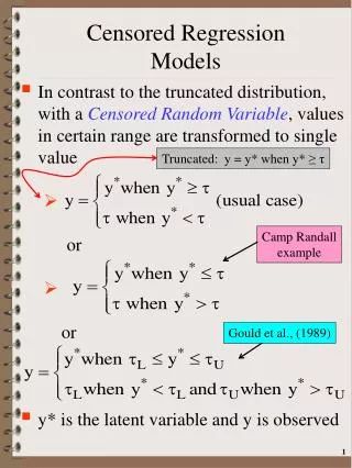
Censored and Truncated Regression Models y = Xβ + ε, ε~N(0,σ2) • Lets relax the CRM assumption that the distribution of y, our dependent variable, is smooth and continuous from ±∞ • Two types of dependent variable distributions: • CensoredRV: Observe dependent variable for entire sample • Values in a certain range are reported as a single value or • There is a significant clustering around a particular value (e.g., 0 acres using conservation tillage) • Truncated RV: Severely limits data • Exclude observations based on characteristics of the dependent variable
Example of Censored Distribution:Demand for Tickets to UW Football Interested in examining demand for tickets but only observe tickets sold. Pdf(Ticket Demand) Pr(Demand< Capacity) Pr(Demand) > Capacity Stadium Capacity C* Seats Demanded Think of ticket demand as being a latent variable as the UW can’t sell more than Camp Randall capacity
Example of Censored Distribution:Sale of Tickets to UW Football Pdf(Ticket Demand) Pr(Demand > Cap.) = area to the right of C* under original PDF Pr(Demand< Capacity) Capacity C* Seats Demanded Note: PDF of ticket demand(in contrast to tickets sold) is a mixture of discrete and continuous distributions (censored distribution)
Censored and Truncated Regression Models • Example of Truncated Distribution • Hausman and Wise (1977): NJ Negative Income Tax Experiment • Low income households are given a tax “rebate” • Rebate increases the more a household earns • Households with earnings more than (1.5 * poverty income level) not included in their sample • yi* =Xiβ + εi< Li → included yi* =Xiβ + εi> Li → excluded • Implies a truncated (from above) distribution of ln(Earnings) which was their dependent variable
Censored and Truncated Regression Models • Hausmanand Wise (1977): NJ Negative Income Tax Experiment • Sample design: • Male, 18-58, able to work, not a full time student or in military had to be present • Family had to have at least 2 members • 1,357 families enrolled out of 50,000 families in Trenton, Paterson-Passaic, Jersey City and Scranton (PA) • Cut-off points Family SizeCut-off 2 $3,195 3 $3,915 4 $5,002 5 $5,895 6 $6,615 7 $7,387 8 $8,160
Censored and Truncated Regression Models • Hausmanand Wise (1977): NJ Negative Income Tax Experiment • What is the issue? • Solid line: average relationship between education and earnings • Dots represent the distribution of earnings around this mean • Assuming the same family size, all individuals w/earnings > L dropped
Censored and Truncated Regression Models • Hausmanand Wise (1977): NJ Negative Income Tax Experiment • Estimated regression underestimates the effect of education on earnings • Sample selection procedure introduces correlation between RHS variables and the error term and leads to biased parameter estimates
Censored and Truncated Regression Models • Hausmanand Wise (1977): NJ Negative Income Tax Experiment • The magnitude of the bias depends on L, β, σ2 and the value of X
Censored and Truncated Regression Models • Example of Truncated (From Above) Distribution CDF(I*) < 1.0 I* i.e., 1.5* Poverty Level
Censored and Truncated Regression Models • Example of Truncated (From Below) Distribution • Contrast the above with the censored distribution shown previously where area under PDF plus PMF = 1.0 Pr(Y > τ) < 1.0 τ
Truncated Regression Models • Assume y has a truncated normal distribution and y*~N(, 2) • y* is latent & y is observed • Assuming lower truncation y = y* | y* > τ (mapping of y from y*) • A truncated density for y is created by dividing original latent y* PDF by the area to the right of truncation point • Forces the area under truncated distribution to = 1.0 (Theorem 24.1, Greene p.864) Note: Regression is a conditional mean generating function Observed value PDF of y*
Truncated Regression Models • The above follows from the definition of a conditional probability
Example of Truncated Distribution (Truncation from Below) y = y* | y* > τ Density f(y|y*>) F(τ) is Pr(y*<τ) F() f(y*) * • f(y|y* > ) = f(y*)/Pr(y* > ) = f(y*)/[1 - F()] (Theorem 24.1, Greene p.864)
Truncated Regression Models • Lets review the relationship between Normal vs Standard Normal Densities we 1st presented under Discrete Choice • y* ~ N(μ,σ2)→PDF of y*is • PDF of standard normal RV, z μz=0 σz=1 pdf of z pdf of y*
Truncated Regression Models • Characteristics of a truncated normal distribution σ > 0 z
Truncated Regression Models y*~N(μ, σ2) Std. Normal PDF Φ≡Std. Normal CDF
Truncated Regression Models Std. Normal PDF 0 Area to right of purple line Area to left of purple line Area to left of red line
Truncated Regression Models y*~N(μ, σ2) • To summarize: Std. Normal CDF Due to symmetry
Truncated Regression Models y* is latent • Characteristics of truncated normal distribution • Using the above relationships y*~N(μ, σ2) f(y* | μ, σ) Pr(y* > τ) f(y* | μ, σ) Pr(y* > τ)
Truncated Regression Models y* is latent y is observed • Moments of truncated normal dist. (Theorem 24.2, Greene p.866) • y*~N(μ, σ2) and τ a constant • E[y*| truncation]=E[y] = μ + σλ(α) • Var[y*|truncation]=Var[y] = σ2[1−δ(α)] How many S.D.’s is τ from the mean of y*? “Hazard Function” λ(α) a.k.a. the Inverse Mill’s Ratio (IMR)
Truncated Regression Models • Note that with: The above due to standard normal PDF symmetry
Truncated Regression Models y*~N(μ, σ2) • Moments of truncated normal distribution • E[y*| truncation] = μ + σλ(α) • If the truncation is from below • That is we exclude values below a certain value • → the mean of the truncated variable is greater than the original mean with E[y] = μ + σλ(α) . >0 >0 >μ
Truncated Regression Models y*~N(μ, σ2) • Moments of truncated normal distribution • E[y*| truncation] = μ + σλ(α) • If the truncation is from above • That is we exclude values above a certain value • → the mean of the truncated variable is less than the original mean with E[y] = μ + σλ(α) . >0 <0
Truncated Regression Models Depends on truncation y*~N(μ, σ2) • Moments of truncated normal distribution • Var[y*|truncation]=σ2[1 - δ(α)] • Truncation reduces variance compared to untruncated distrubtion variance regardless of the truncation (upper or lower) given that 0 ≤ δ(α) ≤ 1
Example of Truncated Distribution (Truncation from Below) y = y* | y* > τ PDF f(y|y*>) f(y*) * For more detail see Maddala’s Appendix and the theorems in Greene
Truncated Regression Models • Side note on the Inverse Mills Ratio • For the standard normal distribution the IMR gives the mean of a truncated distribution • Specifically, if z*~N(0,1) → E(z | z* > a) = φ(a)/[1 - Φ(a)] std. normal PDF std. normal CDF
Truncated Regression Models • Given the above we are now ready to develop the truncated regression model • Lets assume the following: • yi = yi*if yi* > 0, yi* = Xiβ + εi, εi~N(0,σ2) • Using Theorem 24.2 E(yi| yi* > 0,Xi) = Xiβ + σλi • → E(yi| yi* > 0) > E(yi*) Latent regression Lower Truncation τ E(yi*|Xi) >0 Xiβ Xiβ+σλ
Truncated Regression Models • We can motivate the above via the error term: • yi = yi*if yi* > 0, yi* = Xiβ + εi, ε~N(0,σ2) • yi* > 0 →Xiβ + εi > 0→ εi > −Xiβ • Using Theorem 24.2 E(εi| εi > −Xiβ) = E(εi) + σλ = σλi • E(yi| yi* > 0,Xi) = Xiβ + E(εi| εi> −Xiβ) = Xiβ + σλi τ = 0 E(εi) τ Same result as when looking at E(y|y*>0)
Truncated Regression Models y = y* | y* > 0 yi* = Xiβ + εi f(y|y*>0,X) F(0|X) f(y*|X) 0 Xiβ Xiβ+σλ • Truncated regression model: E(yi| yi* > 0,Xi) = Xiβ + σλi
Truncated Regression Models yi* = Xiβ + εi E(yi| yi* > 0,Xi) = Xiβ + σλi E(εi| εi > −Xiβ) = σλi ≠0 • How do we calculate marginal impacts under the truncated regression model? via quotient rule i = observation k = exog. variable Marginal impact has the same sign as βk
Truncated Regression Models • With and 0 < δi< 1 • →βkoverstates the marginal impact of a change in Xk • Marginal impact will have the same sign as βk • Assuming marginal impact is statistically different from 0. • Don’t forget that δi has all the β’s in its formulation via λi, which complicates the variance of the marginal effect • Do you think the marginal effect has the same formulation with upper truncation?
Truncated Regression Models • What is the bias/inconsistency of using the CRM when y is truncated? • Assume y = y * if y* > 0 where
Truncated Regression Models • Bias/Inconsistency of using the CRM when y is truncated • Given the above, the “correct” regression model is: • Compared to the CRM which omits the term σλi • We can think of εi as: σλi+νi • This implies that Xi is correlated with εi given the definition of λi → Cov(Xi,εi) ≠ 0 • Remember Plim βs= β + Cov(Xi,εi)/Var(y) error term “true” unknown value Omitted variable bias
Truncated Regression Models • ML estimation of Truncated Regression model • Truncated Regression likelihood function is derived from the truncated PDF • We have • Lets assume we have the truncation rule: • We know that:
Truncated Regression Models • If we have τ = 0: • From previous results we have: • If we have τ = 0
Truncated Regression Models • Remember for a CRM with normally distributed errors we have: y* = Xβ + ε where εt~N(0,σ2) • The likelihood for the tth obs. given normality can be obtained from the PDF: • The joint density given T iid observations • Which implies the sample log-likelihood ln(joint density of T values of y*)
Truncated Regression Models • We saw above if τ = 0 and we have lower truncation: • The sample log-likelihood is the sum of the logarithms of these densities assuming iid observations f(yi*) Pr(yi* > 0) =1-Φ([0-Xtβ]/σ) ln(joint density of T1 values of y*) This last term is added to the normal PDF to account for truncation ln(joint probability of being above 0) T1 = No. of obs. > 0
Truncated Regression Models ML Estimation of Truncated Regression Proc Defining Likelihood Function Dep. & Exog. Variables Truncate Data Numerical Gradients Least Squares Starting Values Max. Likelihood Proc. Estimates of , σ2, Θ, LLF Elasticity Estimates
Truncated Regression Models • ML estimation of Truncated Regression model • Canadian FAFH Example • 1996 Canadian Food Expend. Survey • 9,767 Households in full sample • Examine restaurant expenditures • 7,699 had expenditures > 0 (78.8%) • Only include these households → truncated sample • Variables included in the analysis • Household income • Urbanization dummies • Regional dummies • No kids? (1 = no kids) • Full-time dummy • Review of MATLAB Code