Limited Dependent Variables Tobit and Censored Models

1. Limited Dependent Variables Tobit and Censored Models y* = b0 + xb + u, y = max(0,y*)

2. Tobit model for corner solutions • Say y* = xb + u, u|x ~ Normal(0,s2) • But we only observe y = max(0, y*) • A nontrival fraction of observations is equal to zero, but is roughly continuous over positive values • Example: amount of charitable contributions

3. Tobit cont. • The latent variable y* satisfies the CLM assumptions: normal, homoskedastic distributions with linear conditional mean • The density of y given x is the same as the density of y* given x for positive values, however for values of y = 0, we have • P(y = 0|x) = P(y* <0|x) = P(u<-x β|x) • P(y = 0|x) = P(u/σ < -x β/σ |x) = Φ(-xβ/σ) = 1 - Φ(xβ/σ) • u/σhas a standard normal distribution and is independent of x. • The density of y given x is: • (2πσ2)-1/2exp[-(y - xi β)2/(2σ2)] = (1/ σ) f[(y - xi β)/ σ], y >0 P(y = 0|x) =1 - Φ(xβ/σ) • The log-likelihood function is • l(β,σ) = 1(y = 0)log[1-Φ(xβ/σ)] + 1(y >0)log{(1/ σ)f[(y- xi β)/ σ]} • As before, the log-likelihood for a random sample of size n is obtained by summing across all i.

4. Tobit cont. • Tobit model uses MLE to estimate both b and s for this model • Important to realize that b estimates the effect of x on y*, the latent variable, not y • Unless the latent variable y* is what is of interest, can’t just interpret the coefficient

5. Tobit cont. • In Tobit models, two expectations are of particular interest • E(y|y>0,x) and E(y|x) • E(y|x) = P(y>0|x)E(y|y>0,x) = F(xb/s)E(y|y>0,x)(A) • To obtain E(y|y>0,x), we use a result from normally distributed random variables • If z ~N(0,1) then E(z|z>c) = f(c) /[1-F(c)] for any constant c.

6. Tobit cont. • E(y|y>0,x) =xβ + E(u|u>-xβ) = xβ + σE(u/σ|u/σ >-xβ/σ) = xβ + σf(xβ/σ)/F(xb/s) = xβ + σl(xβ/σ) (B) • This equation shows why using OLS only for observations where yi>0 will not always consistently estimate β; essentially, the inverse Mills ratio (l = f(c)/ F(c))is an omitted variable, and it is generally correlated with elements of x. • Combining (A) and (B) gives • E(y|x) = F(xb/s)[xβ + σfl(xβ/σ)]= F(xb/s) xb + σf(xβ/σ)

7. Tobit cont. • This last equation shows that when y follows a Tobit model, E(y|x) is a nonlinear function of x and β. • Predicted values will always be positive—but this comes at a cost. Interpretation is now more complicated compared to a linear model • We can get partial effects using calculus

8. Tobit cont. • ∂E(y|y>0,x)/∂xj = bj{1-l(xb/s)[xb/s+l(xb/s)]} • ∂E(y|x)/∂xj = bj F(xb /s) • Note that the partial effect of xj is not just dependent on bj • In practice, we must plug in values for the x’s—usually at the mean or some other value of interest.

9. R2 in Tobit • The R2 is the square of the correlation coefficient between yi and ŷi where ŷi = E(y|x=x) = F(xb/s) xb + σf(xβ/σ) • This is motivated by the fact that the usual R2 for OLS is equal to the square correlation the yi and the fitted values. • Stata Example 9-1

10. Specification issues with Tobit • If normality or homoskedasticity fail to hold, the Tobit model may be meaningless • These two assumptions are crucial—if either fails you should not use Tobit (though, minor departures may be ok)

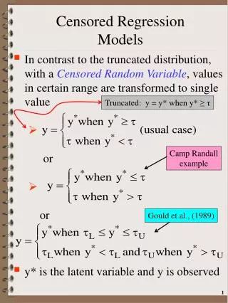
11. Censored Regression Models • More general latent variable models can also be estimated, say • y = xb + u, u|x,c ~ Normal(0,s 2), but we only observe w = min(y,c) if right censored, or w = max(y,c) if left censored • Very common in survey data • For example: Income data often comes in the following form • $0 - $1000, $1001-$2000, …, $100,000 + • We know people in the top category have income greater than $100,000 but we don’t know how much their income is because the data is “top-coded” • w = min($200,000, $100,000) = $100,000

12. Censored Data

13. Censored Data • We should be clear as to how this is different from a Tobit application, for example. In Tobit, there is no issue of data observability, we see all values of the dependent variable: it is simply the case that a nontrivial fraction of them equal zero (or some other upper or lower limit) • The problem that necessitates a censored regression model is one of data observability or missing data. We simply do not see the variable above a certain threshold due to survey design or institutional constraints.

14. Censored Data • We can estimate β by ML given a random sample on (xi, wi). For this, we need the density of wi given (xi, ci). • For uncensored observations, wi = yi and the density of wi is the same as that for yi: N(xi β, σ2). • For censored observations, we need the probability that wi equals ci, given xi: P(wi= ci|xi) = P(yi≥ci-xi β) = 1-Φ[(ci-xiβ/σ)]

15. Censored Data • Combining these two parts to obtain the density of wi, given xi and ci gives us: • f(w|xi, ci) = 1-Φ[(ci-xiβ/σ)] , w = ci = (1/σ) f[(w-xi β)/σ], w < ci • The log likelihood is obtained by taking the natural log of the density for each i. As before, we can maximize the sum of these across i, with respect to βj and σ to get the MLEs. • The good news here is that we can interpret the coefficients directly—just as in OLS.

16. Censored Data • Important to emphasize that we are talking about censoring of the dependent variable. • Censoring on the independent variables may cause efficiency problems but not bias. May also not want to extrapolate too much to values of the independent variables that are beyond the scope of the data

17. Censored Data • One of the most important applications of censored regression models is duration analysis • A duration is a variable that measures the time before a certain event occurs. • For example, we might wish to explain the number of days before a felon released from prison is arrested again. For some felons, this may never happen, or, it may happen after such a long time that we must censor the duration in order to analyze the data. • Stata Example 9-2