Download
1 / 22
220 likes | 375 Vues
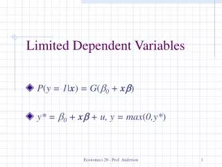
Limited Dependent Variables LPM, Probit and Logit. P ( y = 1| x ) = G ( b 0 + x b ). Limted Dependent Variables (LDV). An LDV is broadly defined as a dependent variable whose range of values is substantially restricted.

E N D
Limited Dependent Variables LPM, Probit and Logit P(y = 1|x) = G(b0 + xb)
Limted Dependent Variables (LDV) • An LDV is broadly defined as a dependent variable whose range of values is substantially restricted. • Participation percentage in a retirement plan must be restricted between 0 and 100 % • The number of times a person has been arrested; 1, 2, 3, … • Did a person smoke marijuana or not (1 = yes, 0 = no)?
LDV, cont. • Many economic variables are limited in some way, often because they must be positive • Wages • Housing prices • Nominal interest rates • If a strictly positive variable takes on many values, a special econometric model is rarely necessary
Binary Dependent Variables • Binary dependent variables generally take the value 1 or 0. • Recall the linear probability model, which can be written as P(y = 1|x) = b0 + xb • A drawback to the linear probability model is that predicted values are not constrained to be between 0 and 1 • An alternative is to model the probability as a function, G(b0 + xb), where 0<G(z)<1
The Probit Model • One choice for G(z) is the standard normal cumulative distribution function (cdf) • G(z) = F(z) ≡ ∫f(v)dv, where f(z) is the standard normal • f(z) = (2p)-1/2exp(-z2/2) • This case is referred to as a probit model • This choice of G ensures that P(y=1|x) will always be between 0 and 1. • Since it is a nonlinear model, it cannot be estimated by our usual methods, instead we will use something called maximum likelihood estimation
The Logit Model • Another common choice for G(z) is the logistic function, which is the cdf for a standard logistic random variable • G(z) = exp(z)/[1 + exp(z)] = L(z) • This case is referred to as a logit model, or sometimes as a logistic regression • Both functions have similar shapes – they are increasing in z, most quickly around 0
Probits and Logits • Both the probit and logit are nonlinear and require maximum likelihood estimation • No real reason to prefer one over the other • Traditionally saw more of the logit, mainly because the logistic function leads to a more easily computed model • Today, probit is easy to compute with standard packages, so more popular
Interpretation of Probits and Logits (vs LPM) • In general we care about the effect of x on P(y = 1|x), that is, we care about ∂p/ ∂x • For the linear case, this is easily computed as the coefficient on x • P(y = 1|x1) = b0 + bx1and ∂p/ ∂x =b • suppose b = .05 and x1 is a variable measured in $. How do we interpret the coefficient on x1?
Interpretation of Probits and Logits (continuous variables) • For the nonlinear probit and logit models with continuous explanatory variables: • ∂p(x)/ ∂xj = g(b0 +xb)bj, where g(z) is dG/dz • This derivative shows that the relative effects of any two continuous explanatory variables do not depend on x: the ratio of the partial effects for xj and xh is • ∂p(x)/ ∂xj = g(b0 +xb)bj =bj ∂p(x)/ ∂xh g(b0 +xb)bhbh
Interpretation of Probits and Logits (binary variables) • Consider the case when you want to evaluate the effect of a job training program on employment (y is binary = 1 if person is employed, zero otherwise and x = 1 if person went to a job training program, zero otherwise). Note: ignore endogeneity of job training program for now • In a linear model, we know just to look at the coefficient on x to obtain a measurement of the effect of job training program • y = b0 + bx • In the probit case, we need to evaluate • G(b0 + b) - G(b0) • What is the interpretation? • In the logit case, we need to evaluate • exp(b0 + b)/[1+ exp(b0 + b)] - exp(b0)/[1+ exp(b0)] • What is the interpretation?
Interpretation (cont.) • Note that knowing the sign of b is enough to know if the effect is positive or negative, but to find the magnitude of the effect, you have to estimate the equations on the previous slide. • With continuous x’s, to compare the magnitude of effects, need to calculate the derivatives, say at the means • Clear that it’s incorrect to just compare the coefficients across the three models (LPM, Logit and Probit) • Can compare sign and significance (based on a standard t test) of coefficients, though • A rule of thumb is to divide probit estimates by 2.5 and logit estimates by 4 to make them comparable to LPM estimates.
Interpretation (cont.) • The biggest difference between the LPM model and the logit/probit models is that the LPM assumes a constant marginal effect, whereas the logit/probit take into account the specific values of the x variables
Maximum Likelihood Estimation (MLE) • Because of the nonlinear nature of these models, OLS is no longer appropriate • The idea behind ML is to provide a way of choosing an asympotically efficient estimator for a set of parameters
Some intuition on ML* • Suppose you have a coin and you want to estimate the probability (call it “p”) that it lands on Heads. You are told that this probability is either 1/2 or 9/10. You toss the coin 10 times and obtain the following sequence: HTHHHTHTHH (7 heads out of 10). What is the maximum likelihood estimate of p? *Credit to Daniele Passerman for this example
Intuition on ML, cont • If the true value of p were 1/2, what is the probability (the likelihood) of observing the sequence that we actually observed? What is the likelihood if p = 9/10? Which of these two values of p is more likely? • The calculations are simple: we just need to use the formula for calculating the probability of observing a given number of successes in a sequence of n Bernoulli trials where the probability of success is equal to p. Let y = 1 if the outcome of trial i was a success and 0 otherwise. The probability of observing k successes is:
Intuition on ML, cont • Plugging in our potential candidates, we get:
Intuition on ML, cont • Thus, it is more likely that the true probability was p = 1/2. This is our MLE. • This simple example shows what we need for ML estimation: • Function for telling us the probability of observing what we actually observe for a given value of the parameters of interest • The parameter space (in our example it was 1/2 and 9/10.) • Then, all we have to do is find the value in the parameter space that maximizes the likelihood function
MLE • Suppose we have a random sample of size n. To obtain the MLE, conditional on the explanatory variables, we need the density of yi given xi: • f(y|xi;b) = [G(xi b)]y[1-G(xi b)]1-y, y = 0,1 • When y = 1, we get • [G(xi b)] • When y = 0, we get • [1-G(xi b)] • The log-likelihood function for observation i is a function of the parameters and the data (xi ,y) and is obtained by taking the log of the equation above: • li(b) = yilog[G(xi b)]+(1-yi)log[1- G(xi b)]
MLE • Because G(.) is between 0 and 1 for logit and probit models, li(b) is well defined for all values of b. • The log-likelihood for a sample size of n is obtained by summing up li(b) across all observations: • L(b) = Σili(b) • We find the b that maximizes this function • Stata Example 8-1
The Likelihood Ratio Test • Unlike the LPM, where we can compute F statistics or LM statistics to test exclusion restrictions, we need a new type of test • Maximum likelihood estimation (MLE), will always produce a log-likelihood, L • Because the MLE maximizes the log-likelihood function, dropping variables generally leads to a smaller log-likelihood. • Just as in an F test, you estimate the restricted and unrestricted model, then form • LR = 2(Lur – Lr) ~ c2q • This will always be positive • Stata Example 8-1, cont.
Goodness of Fit • Unlike the LPM, where we can compute an R2 to judge goodness of fit, we need new measures of goodness of fit • One possibility is a pseudo R2 based on the log likelihood and defined as 1 – Lur/Lr • Can also look at the percent correctly predicted • if predict a probability >.5 then that matches y = 1 and vice versa • Stata Example 8-1, continued