Download
1 / 10
110 likes | 264 Vues
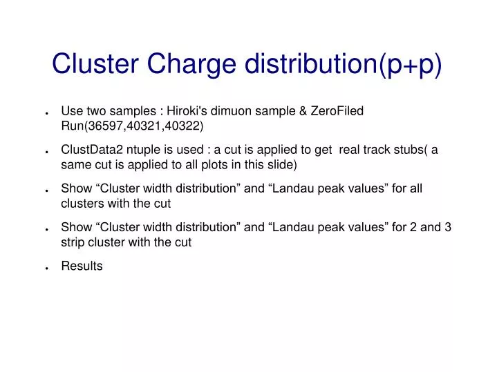
Cluster Charge distribution(p+p). Use two samples : Hiroki's dimuon sample & ZeroFiled Run(36597,40321,40322) ClustData2 ntuple is used : a cut is applied to get real track stubs( a same cut is applied to all plots in this slide)

E N D
Cluster Charge distribution(p+p) • Use two samples : Hiroki's dimuon sample & ZeroFiled Run(36597,40321,40322) • ClustData2 ntuple is used : a cut is applied to get real track stubs( a same cut is applied to all plots in this slide) • Show “Cluster width distribution” and “Landau peak values” for all clusters with the cut • Show “Cluster width distribution” and “Landau peak values” for 2 and 3 strip cluster with the cut • Results
Applied Cut to get real track stubs • Cut ( ClustData2 ntuple ) • bbcvert>-1000 • (lastpl==4) (roadhits>=9 ) && (nroads==1||nroads==2) • one hit per plane • |atan(dx/dz)|<0.17 &&|atan(dy/dz)|<0.17
Cluster width Distribution & Landau Peak value( I ) Slide6 Slide7 and 8 Pla0(ST1) Pla1(ST1) Pla3(ST1) Pla2(ST1) Red : Dimuon sample Blue : ZeroField Count Pla6(ST2) Pla4(ST1) Pla5(ST1) Pla12(ST3) Cluster width • All clusters after the following cut • Error bar : sigma from Landau fitting • Cut ( ClustData2 ntuple ) : no cluster width cut (bbcvert>-1000) && (lastpl==4) && (roadhits>=9 ) && (nroads==1||nroads==2) && (nhits1<=1 && nhits2<=1 && nhits3<=1 && nhits4<=1 && nhits5<=1 && nhits6<=1 )&&(abs(atan(pf2))<0.17&&abs(atan(pf4))<0.17) )
Landau peak vs Plane # w.r.t cluster width(II) Slide10 Slide9 Blue : cluster width = 3 Red : cluster width = 2 Blue : cluster width = 3 Red : cluster width = 2 Hiroki's Dimuon Sample Zero Field • 2 and 3 strip clusters after the following cut • Error bar : sigma from Landau fitting • Cut ( ClustData2 ntuple ) (bbcvert>-1000) && (lastpl==4) && (roadhits>=9 ) && (nroads==1||nroads==2) && (nhits1<=1 && nhits2<=1 && nhits3<=1 && nhits4<=1 && nhits5<=1 && nhits6<=1 )&&(abs(atan(pf2))<0.17&&abs(atan(pf4))<0.17) )
Results • A cut was applied to get real tracks stubs from ClustData2 ntuples • 2 strips clusters are dominant compared with 3 strips clusters • The gain in Station 3 is lower than the other stations • Landau peak values varies with regard to cluster width(2,3), those for 3 strip clusters are a little higher in ST1 and ST3, however much higher in ST2 • What is going on (?) • See the detail informations (Backup slides)(from slide6)
Cluster width distribution Zero Field Hiroki's Dimuon Sample
Cluster Charge(I) & Landau peak : Dimuon Sample ( (bbcvert>-1000) && (lastpl==4) && (roadhits>=9 ) && (nroads==1||nroads==2) && (nhits1<=1 && nhits2<=1 && nhits3<=1 && nhits4<=1 && nhits5<=1 && nhits6<=1 )&&(abs(atan(pf2))<0.17&&abs(atan(pf4))<0.17) ) No cluster width cut
Cluster Charge(I) & Landau peak: ZeroField ( (bbcvert>-1000) && (lastpl==4) && (roadhits>=9 ) && (nroads==1||nroads==2) && (nhits1<=1 && nhits2<=1 && nhits3<=1 && nhits4<=1 && nhits5<=1 && nhits6<=1 )&&(abs(atan(pf2))<0.17&&abs(atan(pf4))<0.17) ) No cluster width cut
Cluster charge (II) : Dimuon sample Cluster width = 3 Cluster width = 2
Cluster charge (II) : Zero Field Run Cluster width = 2 Cluster width = 3


![Cumulative distribution [%]](https://cdn1.slideserve.com/2142714/slide1-dt.jpg)