Download
1 / 19
190 likes | 293 Vues
Mining for Patterns Based on Contingency Tables by KL-Miner First Experience. Jan Rauch Milan Šimůnek (PhD. student) Václav Lín (student) University of Economics Prague. … KL-Miner , First Experience. KL-Miner Basic features Application example Implementation principles

E N D
Mining for Patterns Based on Contingency Tables by KL-Miner First Experience Jan Rauch Milan Šimůnek (PhD. student) Václav Lín (student) University of Economics Prague
… KL-Miner, First Experience • KL-Miner Basic features • Application example • Implementation principles • Scalability • Concluding remarks FDM 2003
KL-Miner -- Data and Patterns Data: Data Matrix • Patterns i.e. KL-hypothesis: R C / • row attribute R {A1, …, AP}, possible values i.e. categories: r1, …, rK • column attribute C {A1, …, AP}, possible values i.e. categories: c1, …,cL • Boolean attribute derived from other attributes A1, …, AP • KL quantifier …. Condition imposed on contingency table of R and C FDM 2003
KL – quantifiers Contingency table of R and C: Examples of quantifiers: Simple aggregate function: Kendall’s quantifier: e.g. |b | P FDM 2003
Kendall’s quantifier Kendall’s coeficient: : b 0;1 b> 0 … positive ordinal dependence b< 0 … negative ordinal dependence b= 0 … ordinal independence |b | = 1 … C is a function of R Kendall’s quantifier: e. g. | b | p or | b | p FDM 2003
KL-Miner application example STULONG Project, 1419 patients, entry examination See http://euromise.vse.cz FDM 2003
STULONG attributes examples (1) Systolic blood pressure Smoking Group of patients FDM 2003
STULONG attributes examples (2) Skinfold above musculus triceps (mm) Beer – amount / day 219 attributes total 38 ordinal attributes We use 17 ordinal attributes FDM 2003
Example - analytic question Are there any ordinal dependencies among attributes under some conditions? at least 50 patients |b | 0.75 relevant conditions : FDM 2003
Example – relevant condition specification (1) Group of patients (normal), Group of patients (risk), … Beer 10(yes), Beer 12(yes), …, Beer 10(yes) Beer 12(yes) Sliding windows … FDM 2003
Example – relevant condition specification (2) Sliding window 4, 5, 6, 7, 9,10, 11, 12, 13, 14, 15, ....., 43, 44, 45, 46, 47, 48, 49, 50 4, 5, 6, 7, 9,10, 11, 12, 13, 14, 15, ....., 43, 44, 45, 46, 47, 48, 49, 50 4, 5, 6, 7, 9,10, 11, 12, 13, 14, 15, ....., 43, 44, 45, 46, 47, 48, 49, 50 ........... 4, 5, 6, 7, 9, 10, 11, 12, 13, 14, 15, ....., 43, 44, 45, 46, 47, 48, 49, 50 4, 5, 6, 7, 9, 10, 11, 12, 13, 14, 15, ....., 43, 44, 45, 46, 47, 48, 49, 50 FDM 2003
Example – output overview 2 min 1sec 550 310 verifications 25 hypotheses 3.06 GHz 512 MB DDR SDRAM FDM 2003
Example – output detail (1) b= 0.82 (i.e. strong positive ordinal dependence) FDM 2003
Example – output detail (2) b= 0.78 (i.e. strong positive ordinal dependence) FDM 2003
Implementation principles (1) Attributes are represented by cards of categories i.e. strings of bits Attributes Cards of categories of A1 FDM 2003
Implementation principles (2) CARD [] = bit string representation of Booelan attribute CARD [ Group of patients (normal) Beer 10(yes) Beer 12(yes) ] = Group of patients [normal] Beer 10[yes] Beer 12[yes] Count() – number of “1” in the bit string FDM 2003
Implementation principles (3) n1,1 = Count( R[r1] C[c1] CARD []) FDM 2003
Scalability 75 000 verifications approximately linear FDM 2003
Concluding remarks • KL-Miner practically interesting results • Suitable for interactive work • Further quantifiers • Combinations with further mining procedures FDM 2003