Download
1 / 44
440 likes | 508 Vues
Program Analysis. Mooly Sagiv http://www.math.tau.ac.il/~sagiv/courses/pa01.html Tel Aviv University 640-6706 Textbook: Principles of Program Analysis Chapter 1.5-8 (modified). Outline. Mathematical Background Abstract Interpretation Type systems Conclusions. Mathematical Background.

E N D
Program Analysis Mooly Sagiv http://www.math.tau.ac.il/~sagiv/courses/pa01.html Tel Aviv University 640-6706 Textbook: Principles of Program Analysis Chapter 1.5-8 (modified)
Outline • Mathematical Background • Abstract Interpretation • Type systems • Conclusions
Mathematical Background • Declaratively define • The result of the analysis • The exact solution • Allow comparison
Posets • A partial ordering is a binary relation : L L {false, true} • For all l L : l l (Reflexive) • For all l1, l2, l3 L : l1 l2, l2 l3 l1 l3 (Transitive) • For all l1, l2 L : l1 l2, l2 l1 l1 = l2 (Anti-Symmetric) • Denoted by (L, ) • In program analysis • l1 l2 l1 is more precise than l2 l1 represents fewer concrete states than l2 • Examples • Total orders (N, ) • Powersets (P(S), ) • Powersets (P(S), ) • More notations • l1 l2 l2 l1 • l1 l2 l1 l2 l1 l2 • l1 l2 l2 l1
Upper and Lower Bounds • Consider a poset (L, ) • A subset L’ L has a lower bound l L if for all l’ L’ : l l’ • A subset L’ L has an upper bound u L if for all l’ L’ : l’ u • A greatest lower bound of a subset L’ L is a lower bound l0 L such that l l0 for any lower bound l of L’ • A lowest upper bound of a subset L’ L is an upper bound u0 L such that u0 u for any upper bound u of L’ • For every subset L’ L: • The greatest lower bound of L’ is unique if at all exists • L’ (meet)a b • The lowest upper bound of L’ is unique if at all exists • L’ (join) ab
Complete Lattices • A poset (L, ) is a complete lattice if every subset has least and upper bounds • L = (L, ) = (L, , , , , ) • = = L • = L = • Lemma For every poset (L, ) the following conditions are equivalent • L is a complete lattice • Every subset of L has a least upper bound • Every subset of L has a greatest lower bound
Cartesian Products • A complete lattice (L1, 1) = (L1, , 1, 1, 1, 1) • A complete lattice (L2, 2) = (, , 2, 2, 2, 2) • Define a Poset L = (L1 L2 ,) where • (x1, x2) (y1, y2) if • x1 x2 and • y1 y2 • L is a complete lattice
Chains • A subset Y L in a poset (L, ) is a chain if every two elements in Y are ordered • For all l1, l2 Y: l1 l2 or l2 l1 • An ascending chain is a sequence of values • l1 l2 l3 … • A strictly ascending chain is a sequence of values • l1 l2 l3… • A descending chain is a sequence of values • l1 l2 l3 … • A strictly descending chain is a sequence of values • l1 l2 l3 … • L has a finite height if every chain in L is finite • Lemma A poset (L, ) has finite height if and only if every strictly decreasing and strictly increasing chains are finite
Monotone Functions • A poset (L, ) • A function f: L L is monotoneif for every l1, l2 L: • l1 l2 f(l1 ) f(l2)
f() f2() Fix(f) Red(f) f2() Ext(f) f() Fixed Points • A monotone function f: L L where (L, , , , , ) is a complete lattice • Fix(f) = { l: l L, f(l) = l} • Red(f) = {l: l L, f(l) l} • Ext(f) = {l: l L, l f(l)} • l1 l2 f(l1 ) f(l2) • Tarski’s Theorem 1955: if f is monotone then: • lfp(f) = Fix(f) = Red(f) Fix(f) • gfp(f) = Fix(f) = Ext(f) Fix(f) gfp(f) lfp(f)
Chaotic Iterations • A lattice L = (L, , , , , ) with finite strictly increasing chains • Ln = L L … L • A monotone function f: LnLn • Compute lfp(f) • The simultaneous least fixed of the system {x[i] = fi(x) : 1 i n } for i :=1 to n do x[i] = WL = {1, 2, …, n} while (WL ) do select and remove an element i WL new := fi(x) if (new x[i]) then x[i] := new; Add all the indexes that directly depends on i to WL x := (, , …, ) while (f(x) x ) do x := f(x)
The Abstract Interpretation Technique • The foundation of program analysis • Goals • Establish soundness of (find faults in) a given program analysis algorithm • Design new program analysis algorithms • The main ideas: • Relate each step in the algorithm to a step in a structural semantics • Establish global correctness using a general theorem • Not limited to a particular form of analysis
Soundness in Reaching Definitions • Every reachable definition is detected • May include more definitions • Less constants may be identified • Not all the loop invariant code will be identified • May warn against uninitailzed variables that are in fact in initialized • At every elementary block lRDentry(l) includes all the possibly definitions reaching l • At every elementary block lRDentry(l) “represents” all the possible concrete states arising when the structural operational semantics reaches l
Proof of Soundness • Define an “appropriate” structural operational semantics • Define “collecting” structural operational semantics • Establish a Galois connection between collecting states and reaching definitions • (Local correctness) Show that the abstract interpretation of every atomic statement is soundw.r.t. the collecting semantics • (Global correctness) Conclude that the analysis is sound CC1976
Structural Operational Semantics to justify Reaching Definitions • Normal states [Var* Z] are not enough • Instrumented states[Var* Z] [Var* Lab*] • For an instrumented state (s, def) and variable xdef(x) holds the last definition of x
[comp1sos] <S1 , (s, d)> <S’1, (s’, d’)> <S1; S2, (s, d)> < S’1; S2, (s’, d’)> [comp2sos] <S1 , (s, d)> (s’, d’) <S1; S2, (s, d)> < S2, (s’, d’)> Instrumented Structural Semantics for While [asssos] <[x := a]l, (s, d)> (s[x Aas], d(x l)) [skipsos] <[skip]l, (s, d)> (s, d) axioms rules
[ifttsos] <if [b]l then S1 else S2, (s, d)> <S1, (s, d)> [ifffsos] <if [b]l then S1 else S2, (s, d)> <S2, (s, d)> if Bbs=tt if Bbs=ff Instrumented Structural Semantics if construct
Instrumented Structural Semanticswhile construct [whilesos] <while [b]l do S, (s, d)> <if [b]l then (S; while [b]l do S) else skip, (s, d)>
The Factorial Program [y := x]1;[z := 1]2; while [y>1]3 do ( [z:= z * y]4; [y := y - 1]5; ) [y := 0]6;
Code Instrumentation • Alternative instrumentation • Generate an equivalent program which maintains more information • Use standard structural operational semantics
Other Consumers of Instrumentation • Specialized interpreters • Code Instrumentation • Performance analysis qpt • count the number of executions of basic blocks or the number of calls to a function • Profiling Tools • Find “hot” paths (paths that are executed often) by remembering which edge in the control flow graph was executed • Cleanness Tools Purify, Insure • identify uninitialized objects
Collecting (Instrumented) Semantics • The input state is not known at compile-time • “Collect” all the (instrumented) states for all possible inputs to the program • No lost of precision
Flow Information for While • Associate labels with program statements describing when statements begin and end • init:StmLab* • init([x := a]l)= l • init([skip]l)= l • init(S1 ; S2) = init(S1) • init(if [b]lthen S1else S2) = l • init(while [b]l do S) = l • final:StmP(Lab*) • final([x := a]l)= {l} • final([skip]l)= {l} • final(S1 ; S2) = final(S2) • final(if [b]lthen S1else S2) = final(S1) final(S2) • final(while [b]l do S) = {l}
Collecting (Instrumented) Semantics(Cont) • The input state is not known at compile-time • “Collect” all the (instrumented) states for all possible inputs to the program • Define d?:Var* Lab* by d?(x)=? • CSentry(l) = {(s’, d’)|s0: (P, (s0, d?) * (S’, (s’, d’)), init(S’)=l} • Soundness w.r.t. operational semanticsFor all (s’, d’) in CSentry (l) For all variable x (x, d(l)) RDentry(l) • Optimality w.r.t. operational semantics
The Factorial Program [y := x]1;[z := 1]2; while [y>1]3 do ( [z:= z * y]4; [y := y - 1]5; ) [y := 0]6;
An “Iterative” Definition • Generate a system of monotonic equations • The least solution is well-defined • The least solution is the collecting interpretation
Equations Generated for Collecting Interpretation • Equations for elementary statements • [skip]lCSexit(1) = CSentry(l) • [b]lCSexit(1) = CSentry(l) • [x := a]lCSexit(1) = {(s[x Aas], d(x l)) | (s, d) CSentry(l)} • Equations for control flow constructsCSentry(l) = CSexit(l’) l’ immediately precedes l in thecontrol flow graph • An equation for the entryCSentry(1) = {(s0, d?) |s0 Var* Z}
The Least Solution • 12 sets of equationsCSentry(1), …, CSexit (6) • Can be written in vectorial form • The least solution lfp(Fcs) is well-defined • Every component is minimal • Since Fcs is monotonic such a solution always exists • CSentry(l) = {(s’, d’)|s0: (P, (s0, d?) * (S’, (s’, d’)), init(S’)=l} • Simplify the soundness criteria
Operational semantics statement s Set of states Set of states concretization abstraction statement s abstract representation Abstract semantics Abstract (Conservative) interpretation abstract representation
The Abstraction Function • Map collecting states into reaching definitions • The abstraction of an individual state:[Var* Z] [Var* Lab*] P(Var* Lab*)(s,d) = {(x, d(x) | x Var* } • The abstraction of set of states:P([Var* Z] [Var* Lab*]) P(Var* Lab*) (CS) = (s, d) CS (s,d) = = {(x, d(x) | (s, d) CS, x Var* } • Soundness(CSentry (l)) RDentry(l) • Optimality
The Concretization Function • Map reaching definitions into collecting states • The formal meaning of reaching definitions • The concretization: P(Var* Lab*) P([Var* Z] [Var* Lab*]) (RD) = {(s, d) | x Var* :(x, d(x) RD}= = { (s, d) | (s, d) RD} • SoundnessCSentry (l) (RDentry(l)) • Optimality
Galois Connections • The pair of functions (, ) form a Galois connection if: CS P([Var* Z] [Var* Lab*]) RD P(Var* Lab*) (CS) RD iff CS (RD) • Alternatively: CS P([Var* Z] [Var* Lab*]) RD P(Var* Lab*) ( (RD)) RD and CS ((CS)) • and uniquely determine each other
Local Concrete Semantics • For every atomic statement S • S : [Var* Z] [Var* Lab*] [Var* Z] [Var* Lab*] • x := a]l ((s, d)) = (s[x Aas], d(x l)) • skip]l ((s, d)) = (s, d) • b]l ((s, d)) = (s, d)
Local Abstract Semantics • For every atomic statement S • S # : P(Var* Lab*) P(Var* Lab*) • x := a]l #(RD) = (RD - {(x, l’) | l’ Lab }) {(x, l)} • skip]l # (RD) = (RD) • b]l # (RD) = (RD)
Local Soundness • For every atomic statement S show one of the following • ({S(s, d) | (s, d) CS } S# ((CS)) • {S(s, d) | (s, d) (RD)} (S# (RD)) • ({S(s, d) | (s, d) (RD)}) S# (RD) • The above condition implies global soundness [Cousot & Cousot 1976] (CSentry (l)) RDentry(l) CSentry (l) (RDentry(l))
Proof of Soundness (Summary) • Define an “appropriate” structural operational semantics • Define “collecting” structural operational semantics • Establish a Galois connection between collecting states and reaching definitions • (Local correctness) Show that the abstract interpretation of every atomic statement is soundw.r.t. the collecting semantics • (Global correctness) Conclude that the analysis is sound
Induced Analysis (Relatively Optimal) • It is sometimes possible to show that a given analysis is not only sound but optimal w.r.t. the chosen abstraction (but not necessarily optimal) • Define S# (RD) = ({S(s, d) | (s, d) (RD)}) • But this S# may not be computable • Derive (at compiler-generation time) an alternative form for S# • A useful measure to decide if the abstraction must lead to overly imprecise results
Type and Effect Systems • The type of a program expression at a given program point provides a conservative estimation to its value in all the execution paths • A type system provides a syntax directed rules for annotating expressions with types • Simple type inference algorithms are linear • But in Ada, ML, ABC… • But types can also include implementation information such as reaching definitions
Annotated Type Base for Reaching Definitions • S : RD1 RD2if S is executed when the reaching definitions is RD1 it produces reaching definitionsRD2 • Similar to the constraint based approach
[seq] S1 : RD1RD2, S2 : RD2RD3 S1; S2: RD1 RD3 [if] S1 : RD1RD2, S2 : RD1RD2 if [b]l then S1 else S2 : RD1 RD2 Annotated Type Base for Reaching Definitions [ass] [x := a]l’: RD (RD - {{(x, l) | l Lab }) {(x, l’)} [skip] [skip]l: RD RD axioms rules
[wh] S : RD RD while [b]l do S: RD RD Annotated Type Base For Whilewhile construct
[sub] S : RD2RD3 S: RD1 RD4 if RD1RD2 and RD3RD4 Annotated Type Base For Whilesubsumption rule
Not Covered • Effect Systems • Transformations
Conclusions • Three similar techniques • Dataflow analysis • Constraint based approach (a generalization) • Type and effect system (directly deals with the syntax) • Abstract interpretation can be used to show soundness of these methods • But more convenient in the dataflow setting • We are ready for more sophisticated analyses