Download
1 / 43
450 likes | 685 Vues
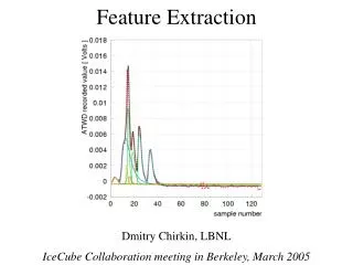
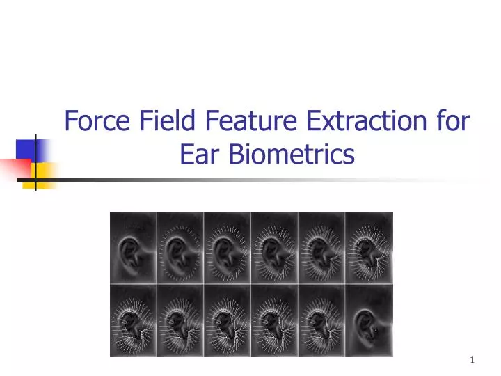
Force Field Feature Extraction for Ear Biometrics. Outline. Introduction Ear topology The force field transforms Force field feature extraction Results Conclusion. Introduction.

E N D
Outline • Introduction • Ear topology • The force field transforms • Force field feature extraction • Results • Conclusion
Introduction The potential of the human ear for personal identification was recognized and advocated as long ago as 1890 by the French criminologist Alphonse Bertillon. In machine vision, ear biometrics has received scant attention compared to the more popular techniques such as automatic face, eye, and fingerprint recognition. Ears have played a significant role in forensic science, especially in the United States, where an ear classification system based on manual measurements has been developed by Iannarelli, and has been in use for more than 40 years. Safety of ear-print evidence has recently been challenged in the Courts.
Introduction Ears have certain advantages over the more established biometrics; as Bertillon pointed out: "The ear, thanks to these multiple small valleys and hills which furrow across it, is the most significant factor from the point of view of identification. Immutable in its form since birth, resistant to the influences of environment and education, this organ remains, during the entire life, like the intangible legacy of heredity and of the intra-uterine life."
Introduction The ear does not suffer from changes in facial expression and is firmly fixed in the middle of the side of the head so that the immediate background is predictable whereas face recognition usually requires the face to be captured against a controlled background.
Method The technique provides a robust and reliable description of the ear without the need for explicit ear extraction. It has two distinct stages: • Image to Force Field Transformation, and • force field Feature Extraction. Firstly, the entire image is transformed into a force field by pretending that each pixel exerts a force on all the other pixels, which is proportional to the pixel's intensity and inversely proportional to the square of the distance to each of the other pixels. It turns out that treating the image in this way is equivalent to passing it through an extremely powerful low pass filter which transforms it into a smooth undulating surface, but with the interesting property that the new surface retains all the original information.
Method Operating in the force field domain allows to access to a wealth of established vector calculus techniques to extract information about this surface. The powerful smoothing also affords valuable resistance to noise and surface matching is also greatly facilitated when the surfaces are smooth. Also, because it is based on a natural force field, there is the prospect of implementing the transform in silicon hardware by mapping the image to an array of electric charges. The smooth surface corresponds to the potential energy field underlying the vector force field and the directional properties of the force field can be exploited to automatically locate a small number of potential wells and channels which correspond to local energy peaks and ridges respectively which then form the basis of the new features.
Method A selection of samples taken from each of sixty-three subjects drawn from the XM2VTS face profiles database has been used to test the viability of the technique.
Outline • Introduction • Ear topology • The force field transforms • Force field feature extraction • Results • Conclusion
Ear Topology The ear does not have a completely random structure, it is made up of standard features just like the face. The parts of the ear are less familiar than the eyes, nose, mouth, and other facial features but nevertheless are always present in a normal ear. These include the outer rim (helix), the ridge (antihelix) that runs inside and parallel to the helix, the lobe, and the distinctive u-shaped notch known as the intertragic notch between the ear hole (meatus) and the lobe. Fig. 1. shows the locations of the anatomical features in detail.
Ear Topology Fig. 1. Topology of the human ear. Just like the face, the ear has standard constituent features consisting of the outer and inner helices, the concha - named for its shell-like appearance, the inter-tragic notch and of course the familiar ear-lobe.
Outline • Introduction • Ear topology • The force field transforms • Force field feature extraction • Ear recognition • Conclusion
Transformation of the image to a force field The image is transformed to a force field by treating the pixels as an array of mutually attracting particles that act as the source of a Gaussian force field, rather like Newton's Law of Universal Gravitation where, for example, the moon and earth attract each other as shown in Fig. 2. Fig. 2. Newton's Universal law of Gravitation. The earth and the moon are mutually attracted according to the product of their masses mE and mM respectively, and inversely proportional to the square of the distance between them. G is the gravitational constant of proportionality.
Transformation of the image to a force field One can use Gaussian force as a generalization of the inverse square laws which govern the gravitational, electrostatic, and magnetostatic force fields, to discourage the notion that any of these forces are in play; the laws governing these forces can all be deduced from Gauss's Law, itself a consequence of the inverse square nature of the forces. Each pixel is assumed to generate a spherically symmetrical force field so that the total force F(rj) exerted on a pixel of unit intensity at the pixel location with position vector rj by a remote pixels with position vector ri and pixel intensities P(ri) is given by the vector summation, In order to calculate the force field for the entire image, this equation should be applied at every pixel position in the image. Units of pixel intensity, force, and distance are arbitrary, as are the co-ordinates of the origin of the vector field.
Transformation of the image to a force field Fig. 3. on the next slide shows an example of the calculation of the force at one pixel location for a simple 9-pixel image. Note that the total force is the vector sum of 8 forces. For an n-pixel image there would be n-1 forces in the summation.
Transformation of the image to a force field Fig. 3. In this simple illustration the force field at the center of a 9-pixel image is calculated by substituting the center pixel with a unit value test pixel and summing the forces exerted on it by the other 8 pixels. In reality, this would not just involve 8 other pixels but hundreds or even thousands of other pixels.
The energy transform for an ear image There is a scalar potential energy field associated with the vector force field where the two fields are related by the equation The force at a given point is equal to the additive inverse of the gradient of the potential energy field at that point. This simple relationship allows the force field to be easily calculated by differentiating the energy field and allows some conclusions drawn about one field to be extended to the other. One can restate the force field formulation in energy terms to derive the energy field equations directly.
The energy transform for an ear image The image is transformed by treating the pixels as an array of particles that act as the source of a Gaussian potential energy field. It is assumed that there is a spherically symmetrical potential energy field generated by each pixel, so that E(rj) is the total potential energy imparted to a pixel of unit intensity at the pixel location with position vector rj by the energy fields of remote pixels with position vectors ri and pixel intensities P(ri), and is given by the scalar summation, where the units of pixel intensity, energy, and distance are arbitrary, as are the co-ordinates of the origin of the field. Fig. 4. show the scalar potential energy field of an isolated test pixel.
The energy transform for an ear image Notice that the highest of the three obvious peaks in previous Fig. has a ridge that slopes gently towards it from the smaller peak to its left. This corresponds to a potential energy channel, because to extend the analogy, water that happened to find its way into its inverted form would gradually flow along the channel towards the peak. The reason for the dome shape of the energy surface can be easily understood by considering the case where the image has just one gray level throughout. In this situation, the energy field at the center would have the greatest share of energy because test pixels at that position would have the shortest average distance between themselves and all the other pixels in the image, whereas test pixels at the corners would have the greatest average distance to all the other pixels, and therefore the least total energy imparted to them.
An Invertible Linear Transform • The transformation is linear since the energy field is derived purely by summation which is itself a linear operation. What is less obvious is that the transform is also invertible.
Outline • Introduction • Ear topology • The force field transforms • Force field feature extraction • Results • Conclusion
Force field Feature Extraction Field line feature extraction is now presented followed by the analytic form of convergence feature extraction. The striking resemblance of convergence to the Marr-Hildreth operator is illustrated and the differences highlighted, especially the nonlinearity of the convergence operator. Note how the features are affected by the combination of the unusual dome shape and changes in image brightness. The close correspondence between the field line and convergence techniques is demonstrated by superimposing their results for an ear.
Field Line Feature Extraction The concept of a unit value exploratory test pixel is exploited to assist with the description field lines. This idea is borrowed from physics, where it is customary to refer to unit value test particles when describing force fields associated with gravitational masses and electrostatic charges. When such notional test pixels are placed in a force field and allowed to follow the field direction their trajectories are said to form field lines. When this process is carried out with many different starting points a set of field lines will be generated that capture the general flow of the force field.
Field Line Feature Extraction Fig. 6. on the next slide demonstrates the field line approach to feature extraction for an ear image, by means of a "lm-strip" consisting of 12 images depicting the evolution of field lines, where each image represents 10 iterations of evolution. The evolution proceeds from top left to bottom right. We see that in the top left image a set of 40 test pixels is arranged in an ellipse shaped array around the ear and allowed to follow the field direction so that their trajectories form field lines describing the flow of the force field.
Fig. 6. Field line, channel, and well formation for an ear. Field line evolution is depicted as a "lm-strip" of 12 images, each depicting 10 iterations of evolution. The top left image shows where 40 test-pixels have been initialized, and the bottom right image shows where 4 wells have been extracted.
Field Line Feature Extraction The test pixel positions are advanced in increments of one pixel width, and test pixel locations are maintained as real numbers, producing a smoother trajectory than if they were constrained to occupy exact pixel grid locations. Notice how ten field lines cross the upper ear rim and how each line joins a common channel that follows the curvature of the ear rim rightwards finally terminating in a potential well. The well locations have been extracted by observing clustering of test pixel co-ordinates so that the bottom right image is simply obtained by plotting the terminal positions of all the co-ordinates.
Dome Shape and Brightness Sensitivity Viewpoint invariance or illumination invariance, either in intensity or direction, is not essential for ear recognition. However, it is still interesting to investigate how the position of features will be affected by the combination of the unusual dome shape and changes in image brightness.
Fig. 7. Effect of additive and multiplicative brightness changes. The original image in (a) has a mean value of 77 and a standard deviation of 47. Images (b) to (d) show the effect of progressively adding offsets of one standard deviation. We see that the channel structure hardly alters and we therefore conclude that operational lighting variation in a controlled biometrics environment will have little effect.
Convergence Feature Extraction An analytical method of feature extraction as opposed to the field line method can be introduced. This method came about as a result of analyzing in detail the mechanism of field line feature extraction. When the arrows usually used to depict a force field are replaced with unit magnitude arrows, thus modeling the directional behavior of exploratory test pixels, one can see that channels and wells arise as a result of patterns of arrows converging towards each other, at the interfaces between regions of almost uniform force direction.
Convergence Feature Extraction As the divergence operator of vector calculus measures precisely the opposite of this effect, it was natural to investigate the nature of any relationship that might exist between channels and wells and this operator. This resulted not only in the discovery of a close correspondence between the two, but also showed that divergence provided extra information corresponding to the interfaces between diverging arrows. "Convergence provides a more general description of channels and wells in the form of a mathematical function in which wells and channels are revealed to be peaks and ridges respectively in the function value."
Convergence Feature Extraction The concept of the divergence of a vector field will first be explained, and then used to define the new function. The function's properties are then analyzed in some detail, and the close correspondence between field line feature extraction and the convergence technique is illustrated by superimposing their results for an ear image.
Convergence Feature Extraction Fig. 9.(b) shows the convergence field for an ear image, while Fig. 9.(a) shows the corresponding field lines. A magnified version of a small section of the force direction field, depicted by a small rectangular insert in Fig. 9.(a), is shown in Fig. 9.(c). In Fig. 9.(b) the convergence values have been adjusted to fall within the range 0 to 255, so that negative convergence values corresponding to antichannels appear as dark bands, and positive values corresponding to channels appear as white bands. Notice that the antichannels are dominated by the channels, and that the antichannels tend to lie within the confines of the channels. Also, notice how wells appear as bright white spots. "The convergence map provides more information than the field lines, in the form of negative versions of wells and channels“.
Convergence Feature Extraction The convergence map provides more information than the field lines, in the form of negative versions of wells and channels or antiwells and antichannels. Although it should be possible to modify the field line technique to extract this extra information by seeding test pixels on a regular grid and reversing the direction of test pixel propagation. Fig. 10. Correspondence between channels and convergence. (a) shows the field line map whilst (b) shows the convergence map and (c) shows the superposition of these two maps where we can see clearly that the channels coincide with the ridges in the convergence map. The technique was validated on a set of 252 ear images taken from 63 subjects selected from the XM2VTS face database achieving almost total correct recognition.
Outline • Introduction • Ear topology • The force field transforms • Force field feature extraction • Results • Conclusion
Experiment results and analysis The force field technique gives a correct classification rate of 99.2% on this set. Running PCA on the same set gives a result of only 62.4%, but when the ears are accurately extracted by cropping to the average ear size of 11173, running PCA then gives a result of 98.4%, thus demonstrating the inherent extraction advantage. The first image of the four samples from each of the 63 subjects was used in forming the PCA covariance matrix. Fig. 12. shows the first 4 eigenvectors for the 111 73-pixel images. The effect of brightness change by addition was also tested where we see that in the worst case where every odd image is subjected to an addition of 3 standard deviations the force field results only change by 2%. whereas those for PCA under the same conditions fall by 36%, or by 16% for normalized intensity PCA, thus confirming that the technique is robust under variable lighting conditions.
Fig. 11. Feature extraction for subject 000 at 141101 pixels. The top row shows the four sample ear images for the subject, whilst the middle row shows the corresponding convergence maps. The bottom row shows the maps after ternary thresholding and also depicts a rectangle centered on the convergence centroid. Notice that the ear image for 000-2 is lower than the others but that the rectangle has correctly tracked it downwards
Fig. 12. shows the first 4 of the 63 eigenvectors for the 111 73-pixel images. The first image of the four samples from each of the 63 subjects was used in forming the PCA covariance matrix.
Outline • Introduction • Ear topology • The force field transforms • Force field feature extraction • Results • Conclusion
Conclusions The lecture presented a new linear transform that transforms an ear image, with very powerful smoothing and without loss of information, into a smooth dome shaped surface whose special shape facilitates a new form of feature extraction that extracts the essential ear signature without the need for explicit ear extraction. Other techniques based on PCA and Force Field Transformation are also discussed. The recognition potential of the human ear for biometrics is yet to be fully established.
References • Hurley, D. J. (2006). Force Field Feature Extraction for Ear Biometrics, World Scientific Review Volume, May 2006. • Messer, K., Matas, J., Kittler, J., Luettin, J., and Maitre, G., (1999). XM2VTSDB: The Extended M2VTS Database, Proc. AVBPA'99 Washington D.C.