Download
1 / 44
440 likes | 597 Vues
Stochastic Gradient Descent and Tree Parameterizations in SLAM. G. Grisetti. Autonomous Intelligent Systems Lab Department of Computer Science, University of Freiburg, Germany. Special thanks to E. Olson, G.D. Tipaldi, S. Grzonka, C. Stachniss, D. Rizzini, B. Steder, W. Burgard, ….

E N D
Stochastic Gradient Descent and Tree Parameterizationsin SLAM G. Grisetti Autonomous Intelligent Systems Lab Department of Computer Science,University of Freiburg, Germany Special thanks to E. Olson, G.D. Tipaldi, S. Grzonka, C. Stachniss, D. Rizzini, B. Steder, W. Burgard, …
What is this Talk about? SLAM localization mapping integrated approaches (SPLAM) active localization exploration path planning [courtesy of Cyrill and Wolfram]
What is “SLAM” ? • Estimate the pose and the map at the same time • SLAM is hard, because • a map is needed for localization and • a good pose estimate is needed for mapping courtesy of Dirk Haehnel
SLAM: Simultaneous Localization and Mapping • Full SLAM: • Online SLAM: Integrations typically done one at a time Estimates entire path and map! Estimates most recent pose and map!
Map Representations • Grid maps or scans [Lu & Milios, `97; Gutmann, `98: Thrun `98; Burgard, `99; Konolige & Gutmann, `00; Thrun, `00; Arras, `99; Haehnel, `01;…] • Landmark-based [Leonard et al., `98; Castelanos et al., `99: Dissanayake et al., `01; Montemerlo et al., `02;…
Path Representations • How to represent the belief about the location of the robot at a given time? • Gaussian • Compact • Analytical Updates • Non multi-modal • Sample-based • Flexible • Multi-modal • Poor representation of large uncertainties • Past estimates cannot be refined in a straightforward fashion
Is the Gaussian a Good Approximation? [Stachniss et al., `07]
Incremental SLAM Gaussian Filter SLAM Smith & Cheesman, `92 Castelanos et al., `99 Dissanayake et al., `01 … Fast-SLAM Haehnel, `01 Montemerlo et al., `03 Grisetti et al., ‘04 … Full SLAM EM Burgard et al., `99 Thrun et al., `98 Graph-SLAM Folkesson et al.,`98 Frese et al.,`03 Howard et al.,`05 Thrun et al.,`05 Our Approach Techniques for Generating Consistent Maps
What This Presentation is About • Estimate the Gaussian posterior of the poses in the path, given an instance of full SLAM problem. • Two Steps: • Estimate the means via nonlinear optimization (maximum likelihood) • Estimate the covariance matrices via belief propagation and covariance intersection
Graph Based Maximum Likelihood Mapping • Goal: • Find the configuration of poses which better explains the set of pairwise observations.
Related Work • 3D approaches: • Nuechter et al., ‘05 • Dellaert et al., ‘05 • Triebel et al., ‘06 • 2D approaches: • Lu and Milios, ‘97 • Montemerlo et al., ‘03 • Howard et al., ‘03 • Dellaert et al., ‘03 • Frese and Duckett, ‘05 • Olson et al., ‘06 • Grisetti et al., ‘07 First to introduce SGD in ML mapping First to introduce the Tree Parameterization
Problem Formulation • The problem can be described by a graph Goal: • Find the assignment of poses to the nodes of the graph which minimizes the negative log likelihood of the observations: Observation of from error nodes
Hessian Information matrix Learning rate Jacobian residual Preconditioned Gradient Descent • Decomposes the overall problem into a set of simple sub-problems. Each constraint is optimized individually. • The magnitude of the correction decreases with each iteration. • A solution is found when an equilibrium is reached. • Update rule for a single constraint: Previous solution Current solution [Olson et al., ’06]
Parameterizations • Transform the problem into a different space so that: • the structure of the problem is exploited. • the calculations become easier and faster. parameters poses Mapping function transformed problem
Tree Parameterization • Construct a spanning tree from the graph. • The mapping function between the poses and the parameters is: • Error of a constraint in the new parameterization. • Only variables in the path of a constraint are involved in the update.
Gradient Descent on a Tree Parameterization • Using a tree parameterization we decompose the problem in many small sub-problems which are either: • constraints on the tree (open loop) • constraints not in the tree (single loop) • Each GD equation independently solves one sub-problem at a time. • The solutions are integrated via the learning rate.
Fast Computation of the Update • 3D rotations lead to a highly nonlinear system. • Update the poses directly according to the GD equation may lead to poor convergence. • This effect increases with the connectivity of the graph. • Key idea in the GD update: Distribute a fraction of the residual along the parameters so that the error of that constraint is reduced.
Fast Computation of the Update The “spirit” of the GD update: • smoothly deform the path along the constraints so that the error is reduced. Distribute the rotations Distribute the translations
Distribution of the Rotational Error • In 3D the rotational error cannot be simply added to the parameters because the rotations are not commutative. • Our goal is to find a set of rotations so that the following equality holds: rotations along the path fraction of the rotational residual in the local frame corrected terms for the rotations
Rotational Error in the Global Reference Frame • We transfer the rotational residual to the global reference frame • We decompose the rotational residual into a chain of incremental rotations obtained by spherical linear interpolation: • And we recursively solve the system
Simulated Experiment • Highly connected graph • Poor initial guess • LU & friends fail • 2200 nodes • 8600 constraints
Real World Experiment The video is accelerated by a factor of 1/50! • 10km long trajectory and 3D lasers recorded with a car • Problem not tractable by standard optimizers
Comparison with Standard Approaches (LU Decomposition) • Tractable subset of the EPFL dataset • Optimization carried out in less than one second. • The approach is so fast that in typical applications one can run it while incrementally constructing the graph.
Incremental Optimization • An incremental version requires to optimize the graph while it is built • The complexity increases with • the size of the graph and with • the quality of the initial guess • We can limit it by • using the previous solution to compute the new one. • refining only portions of the graph which may be altered by the insertion of new constraints. • performing the optimization only when needed. • dropping the information which are not valuable enough. • The problem grows only with the size of the mapped area and not with the time.
Data Association • So far we explained how to compute the mean of the distribution given the data associations. • However, to determine the data associations we need to know the covariance matrices of the nodes. • Standard approaches include: • Matrix inversion • Loopy belief propagation • Belief propagation on spanning tree • Loopy intersection propagation [Tipaldi et al. IROS 07]
Graphical SLAM as a GMRF • Factor the distribution • local potentials • pairwise potentials
Belief Propagation • Inference by local message passing • Iterative process • Collect messages • Send messages B A C D
Belief Propagation - Trees • Exact inference • Message passing • Two iterations • From leaves to root: variable elimination • From root to leaves: back substitution A B C D
Belief Propagation - loops • Approximation • Multiple paths • Overconfidence • Correlations between path A and path B • How to integrate information at D? A B B C A D
Fusion rule for unknown correlations Combine A and B to obtain C Covariance Intersection A B C
Key ideas Exact inference on a spanning tree of the graph Augment the tree with information coming from loops How Approximation by means of cutting matrices Loop information within local potentials (priors) Loopy Intersection Propagation
Approximation via Cutting Matrix • Removal as matrix subtraction • Regular cutting matrix A B C D
Fusing Loops with Spanning Trees • Estimate A and B • Fuse the estimates • Compute the priors A B B C A D
LIP – Algorithm • Compute a spanning tree • Run belief propagation on the tree • For every off-tree edge • compute the off-tree estimates, • compute the new priors, and • delete the edge • Re-run belief propagation
Simulated data Randomly generated networks of different sizes Real data Graph extracted from Intel and ACES dataset from radish Approximation error Frobenius norm Conservativeness Smallest eigenvalue of matrix difference Experiments – Setup & Metrics
Experiments – Simulated Data Approximation error Conservativeness
Experiments – Real Data (Intel) Spanning tree belief propagation Loopy belief propagation Overconfident Too conservative
Experiments – Real Data (Intel) Approximation Error Loopy intersection propagation Conservativeness
Conclusions • Novel algorithm for optimizing 2D and 3D graphs of poses • Error distribution in 2D and 3D and efficient tree parameterization of the nodes • Orders of magnitude faster than standard nonlinear optimization approaches • Easy to implement (~100 lines of c++ code) • Open source implementation available at www.openslam.org • Novel algorithm for computing the covariance matrices of the nodes • Linear time complexity • Tighter estimates • Generally conservative • Applications to both range based and vision based SLAM.