Download
1 / 23
230 likes | 324 Vues
Confounding from Cryptic Relatedness in Association Studies. Benjamin F. Voight (work jointly with JK Pritchard). Importance. Case/control association tests are becoming increasingly popular to identify genes contributing to human disease.

E N D
Confounding from Cryptic Relatedness in Association Studies Benjamin F. Voight (work jointly with JK Pritchard)
Importance • Case/control association tests are becoming increasingly popular to identify genes contributing to human disease. • These tests can be susceptible to false positives if the underlying statistical assumptions are violated, i.e. independence among all sampled alleles used in the test for association. • It is well appreciated that population structure results in false positives (Knowler et al., 1988; Lander and Schork, 1994). • Methods exist which correct for this effect (Devlin and Roeder, 1999; Pritchard and Rosenberg, 1999; Pritchard et al. 2000). • Case/control association tests are becoming increasingly popular to identify genes contributing to human disease. • These tests can be susceptible to false positives if the underlying statistical assumptions are violated, i.e. independence among all sampled alleles used in the test for association. • It is well appreciated that population structure results in false positives (Knowler et al., 1988; Lander and Schork, 1994). • Methods exist which correct for this effect (Devlin and Roeder, 1999; Pritchard and Rosenberg, 1999; Pritchard et al. 2000).
Obtain a sample of affected cases from the population. Your (favorite) Population Obtain a sample of affected cases from the population. Cases are not independent draws from the population allele frequencies. Cases are not independent draws from the population allele frequencies. Problem: the relatedness is cryptic, so the investigator does not know about the relationships in advance. Problem: the relatedness is cryptic, so the investigator does not know about the relationships in advance.
Importance • Devlin and Roeder (1999) have argued that if one is doing a genetic association study, then surely one must believe that the trait of interest has a genetic basis that is at least (partially) shared among affected individuals. • Given that cases share a set of risk factors by descent, then presumably they are more related to one another than to random controls. • These authors presented numerical examples which suggested that this effect may be an important factor, in practice. • However, these examples were artificially constructed, and not modeled on any population-based process. • Few empirical data to suggest if cryptic relatedness negatively impacts association studies. In a founder population, non-independence resulting from relatedness does matter. (Newman et al., 2001). • Devlin and Roeder (1999) have argued that if one is doing a genetic association study, then surely one must believe that the trait of interest has a genetic basis that is at least (partially) shared among affected individuals. • Given that cases share a set of risk factors by descent, then presumably they are more related to one another than to random controls. • These authors presented numerical examples which suggested that this effect may be an important factor, in practice. • However, these examples were artificially constructed, and not modeled on any population-based process. • Few empirical data to suggest if cryptic relatedness negatively impacts association studies. In a founder population, non-independence resulting from relatedness does matter. (Newman et al., 2001).
Goals • Determine whether, or when, cryptic relatedness is likely to be a problem for general applications. • Develop a formal model for cryptic relatedness in a population genetics framework. • In a founder population, estimate the inflation factor due to (cryptic) relatedness, and compare to analytical results. • Avoid staring at “x” in front of a chalkboard. • Determine whether, or when, cryptic relatedness is likely to be a problem for general applications. • Develop a formal model for cryptic relatedness in a population genetics framework. • In a founder population, estimate the inflation factor due to (cryptic) relatedness, and compare to analytical results. • Avoid staring at “x” in front of a chalkboard.
Modeling Definitions • m affected individuals and m random controls, sampled in the current generation. • Pairs of chromosomes coalesce in a previous generation t = 1, 2, … t with the usual probabilities. • All samples are typed at a single bi-allelic locus, unlinked to disease, with alleles B and b, at frequencies p and (1-p) in the population. • m affected individuals and m random controls, sampled in the current generation. • Pairs of chromosomes coalesce in a previous generation t = 1, 2, … t with the usual probabilities. • All samples are typed at a single bi-allelic locus, unlinked to disease, with alleles B and b, at frequencies p and (1-p) in the population. ~ ~
Definitions • Define: • Kp – population prevalence of disease. • Kt – probability that an relative of type t (or t ) of an affected proband is also affected. • lt – recurrence risk ratio, Kt/Kp (Risch, 1990). • Gi(a) – indicator (0 or 1) for the B allele on homologous chromosome a for the i-th case. (with a Î {0, 1} for diploid individuals) • Hj(a) – as above, but for a j-th random control. • Define: • Kp – population prevalence of disease. • Kt – probability that an relative of type t (or t ) of an affected proband is also affected. • lt – recurrence risk ratio, Kt/Kp (Risch, 1990). • Gi(a) – indicator (0 or 1) for the B allele on homologous chromosome a for the i-th case. (with a Î {0, 1} for diploid individuals) • Hj(a) – as above, but for a j-th random control. ~
Define a test statistic which measure the difference in allele counts between cases and controls (slightly modified from Devlin and Roeder, 1999): • Define a test statistic which measure the difference in allele counts between cases and controls (slightly modified from Devlin and Roeder, 1999): • Under the null hypothesis of no association between the marker and phenotype, an allele has a genotype B with probability p, independently for all alleles in the sample. If so, • Under the null hypothesis of no association between the marker and phenotype, an allele has a genotype B with probability p, independently for all alleles in the sample. If so, • If cryptic relatedness exists in the sample, then the variance of the test – call this Var*[T ] – may exceed the variance under the null. We measure the deviation from the null variance using the “inflation factor” d: • If cryptic relatedness exists in the sample, then the variance of the test – call this Var*[T ] – may exceed the variance under the null. We measure the deviation from the null variance using the “inflation factor” d:
Recall that we want the variance to our test, T, under a model of cryptic relatedness: • Recall that we want the variance to our test, T, under a model of cryptic relatedness: • Use the following non-dodgy assumptions: 1. Draws of alleles from the population are simple Bernoulli trials. (Variance terms) 2. Controls are a random sample from the population. (Covariance terms with Hj’s are 0) 3. Allow the possibility that cases and controls depart from Hardy-Weinberg proportions by some factor, call this F. (Covariance terms for alleles in the same individual) 4. For the mutational model, a. Suppose the mutation process is the same for cases and random controls. b. Conditional on a case and random chromosome having a very recent coalescent time (on the order of 1-10 generations), assume that the chance that the alleles are in different states is » 0. • Use the following non-dodgy assumptions: 1. Draws of alleles from the population are simple Bernoulli trials. (Variance terms) 2. Controls are a random sample from the population. (Covariance terms with Hj’s are 0) 3. Allow the possibility that cases and controls depart from Hardy-Weinberg proportions by some factor, call this F. (Covariance terms for alleles in the same individual) 4. For the mutational model, a. Suppose the mutation process is the same for cases and random controls. b. Conditional on a case and random chromosome having a very recent coalescent time (on the order of 1-10 generations), assume that the chance that the alleles are in different states is » 0.
Then after … JKP attempts desperately to keep me honest. Smoke from my brain Me, after many hours of intensive thought processing
Var*[T ] can be simplified to: which denotes the probability that allele copy a and a´from individuals i and i´coalesce in time , conditional on the proposition that individuals i and i´ are both affected (with i≠i´). So what’s this probability? where i≠i´. • And now, we evaluate the covariance term under a model of cryptic relatedness. This covariance term is fairly complicated, but it is related to the following probability:
Depends on the population model (not on phenotype) Depends on the genetic model • Apply some Bayesian Trickery: • … and after some plug and play we finally get:
Under an additive model • Handy relationship between any lr’s and the sibling recurrence risk ratio, a single parameter under an additive model (Risch, 1990): where fr is the kinship coefficient for type-r relatives, which is ¼ for r = 1, and decays by ½ for each increment to r. Using this relationship we can simplify
Simulations • Use Wright-Fisher forward simulation to assess analytical results: • Simulate 1,000 bi-allelic unlinked loci forward in time 4N generations, with mutation parameter q = 4Nm = 1. (†) • Choose a single locus with the desired disease allele frequency, and assign phenotypes to all members of the population under an additive genetic model. • Select m cases and m random controls, use all non-disease loci to infer the inflation factor based on the mean of all tests. (†) because WF simulations are notoriously slow to simulate, we use a speed-up by simulating a smaller population with a proportionally higher mutation rate, and then rescale the population size and mutation rate to the desired levels.
Simulation Results 95% central interval about the mean was at least .001 in each case.
“Tautological” Hutterite Analysis • Quick-note on the Hutterites • 13,000 member pedigree where the genealogy is known, with ~800 members phenotyped/genotyped at many markers across the genome. • Target (for each phenotype): a. Estimate coalescent probabilities for cases and random controls based on the genealogy – “allele-walking” simulations b.Calculate the inflation factor (d) for each phenotype, and compare to the analytic prediction.
Note increased probabilities in cases over random controls for recent coalescent times
Hutterite Analysis • Quick-note on the Hutterites • 13,000 member pedigree where the genealogy is known, with ~800 members phenotyped/genotyped at many markers across the genome. • Target (for each phenotype): a. Estimate coalescent probabilities for cases and random controls based on the genealogy – “allele-walking” simulations b. Calculate the inflation factor (d) for each phenotype, and compare to the analytic prediction.
Empirical d’s in a Founder Population The inbreeding coefficient (F) was estimated at .048 and was included in the calculation.
Summary • We modeled cryptic relatedness using population-based processes. Surprisingly, these expressions are functions of directly observable parameters (population size, sample size, and the genetic model parameterized by lr). • Our analytical results indicate that increased false positives due to cryptic relatedness will usually be negligible for outbred populations. • We applied out technique to a founder population as an example. For six different phenotypes we found evidence for inflation, which matched analytic predictions. • We modeled cryptic relatedness using population-based processes. Surprisingly, these expressions are functions of directly observable parameters (population size, sample size, and the genetic model parameterized by lr). • Our analytical results indicate that increased false positives due to cryptic relatedness will usually be negligible for outbred populations. • We applied out technique to a founder population as an example. For six different phenotypes we found evidence for inflation, which matched analytic predictions.
Acknowledgements • JK Pritchard and NJ Cox (thesis advisors) • Carole Ober (access to the empirical data) • $/£ : NIH, NIH/NIGMS Genetics Training Grant Fine, name that tune: from memory, recite of the first 1677 words of Kingman’s 1982 paper and I’ll get the next round. In the bar at the conference during the week