Download
1 / 21
210 likes | 319 Vues
Tables and Graphs Part II. February 2, 2005. What you can do with Interval/Ratio level data…. Ungrouped ‘ratio’ data. Option #1: Ungrouped Frequency Distribution. A table that displays all the possible values for this variable along with the frequency of occurrence for each value.

E N D
Tables and Graphs Part II February 2, 2005
What you can do with Interval/Ratio level data… • Ungrouped ‘ratio’ data
Option #1: Ungrouped Frequency Distribution • A table that displays all the possible values for this variable along with the frequency of occurrence for each value. • List all values between the minimum and maximum scores in column 1 • Count the number of subjects who obtained each value and place the frequency in column 2. • Columns 3, 4, etc. may include %, cumulative %, cumulative frequency, etc.
Step #3 Compute the % frequency for each value (determines the Mode) How to create an Ungrouped Frequency Distribution Step #4 Compute the cumulative frequency Step #1 List all values between the minimum and maximum scores in column 1. Do not skip any! Step #5 Compute the cumulative percent (determines the Median) Step #2 Count the number of subjects who obtained each value and place the frequency in column 2. Step #6 Create a title for the table… be sure to use APA format.
Grouped Frequency Distribution • A table that displays the frequency of occurrence in “intervals” • The number of intervals should be <15 • Logic and convention play the most important roles when determining the number of intervals
Steps for creating a Grouped Frequency Distribution • Determine range (Range = High Score - Low Score) • Determine interval width • Width=Range/15 • Round the width up or down to a reasonable/logical number • Determine the lowest interval, create mutually exclusive and exhaustive categories • Count the number of scores (f) that fall in each interval • Use the same procedures the were used for creating an ungrouped table
Step #3 Determine the lowest interval, create mutually exclusive and exhaustive categories Grouped frequency distribution for the Honolulu Heart Study Data Range=91-47=44 Step #4 Count the number of scores (f) that fall in each interval Width = 44/15 = 2.9333 Round to 3 Step #1 Determine range (Range = High Score - Low Score) Step #5 Decide if this interval width is the best way to display your data. Modify the table accordingly Choices for lowest interval: 47-49 46-48 45-47 Step #2 Determine interval width Width=Range/15 Round the width up or down
The Stem-and-Leaf Plot • Each number in the data set is broken into two pieces called a stem and a leaf. • Stem • The first part of the number • Consists of the beginning digit(s) • Leaf • The last part of the number • Consists of the final digit(s) Example: 213 (stem=2, leaf=13) or (stem=21, leaf=3)
Matching variables to graphs that represent the raw data values
Cumulative Frequency Distribution (also called an Ogive curve)
For Friday… • Practice • Practice • Practice