Download
1 / 16
190 likes | 512 Vues
Interpolation and Approximation using Radial Base Functions (RBF). Alex Chirokov. Description of rbfcreate and rbfinterp functions. http://www.mathworks.com/matlabcentral/fileexchange/loadFile.do?objectId=10056&objectType=FILE. Outline. First Example Radial Base Functions (RBF)

E N D
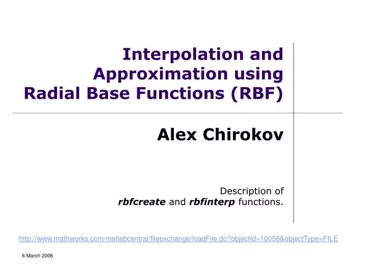
Interpolation and Approximation usingRadial Base Functions (RBF) Alex Chirokov Description of rbfcreate and rbfinterpfunctions. http://www.mathworks.com/matlabcentral/fileexchange/loadFile.do?objectId=10056&objectType=FILE
Outline • First Example • Radial Base Functions (RBF) • RBF Interpolation and Approximation • 1D Examples • 2D Examples
Function: rbfcreate Interpolation coefficients used in function rbfinterp. (output) coeff = rbfcreate(x, y); dim x n matrix of coordinates of the nodes. (input) 1 x n vector of values at the nodes. (input) n - number of nodes dim – dimensionality of the data dim=1 for 1D interpolation, dim=2 for 2D interpolation, etc.
Function: rbfinterp 1 x n vector of values at the nodes. (output) yi = rbfinterp(xi, coeff); dim x m matrix of coordinates of the nodes. (input) Interpolation coefficients created by function rbfcreate. (input) m - number of nodes dim – dimensionality of the data dim=1 for 1D interpolation, dim=2 for 2D interpolation, etc.
First Example 1D Interpolation using standard Matlab function interp1 (see Matlab help on interp1 for detailes): x = 0:1.25:10; y = sin(x); xi = 0:.1:10; yi = interp1(x,y,xi); The same interpolation can be obtained using rbfcreate and rbfinterp functions: x = 0:1.25:10; y = sin(x); xi = 0:.1:10; yi = rbfinterp(xi, rbfcreate(x, y)); Thus for 1D RBF interpolation yi = rbfinterp(xi, rbfcreate(x, y)); can be used instead of yi = interp1(x,y,xi);the rest of the code remains the same.
First Example yi = interp1(x,y,xi); 1D interpolation using RBF and interp is almost identical because default radial base function is linear. Interpolation nodes are shown with ‘o’ symbol. Interpolated data is green, original function is red. yi = rbfinterp(xi, rbfcreate(x, y));
Radial Base Functions A radial basis function (RBF) is a function based on a scalar radius. Functions available in rbfcreate: Gaussian: Multiquadrics: Linear: Gaussian and Multiquadrics functions have adjustable parameter σ. Cubic: Thinplate:
RBF Interpolation The objective of RBF interpolation is to construct the approximation of the function by choosing coefficients C0, C1 and λi to match values of the function at the interpolation nodes. Once coefficients C0, C1 and λi are found. This expression can be used to estimate value of the function at any point.
Radial Base Functions • RBF function can be specified in rbfcreate, if RBF function is not specified linear RBF function is used for interpolation. • Example: • coeff = rbfcreate(x, y,'RBFFunction', 'multiquadric'); • Valid values of 'RBFFunction‘: • 'multiquadric‘ • ‘linear‘ • ‘cubic‘ • ‘gaussian‘ • ‘thinplate‘. Matlab code used to generate Figure on the right x = 0:0.01:3; ym = sqrt(x.*x+1); yg = exp(-x.*x/2); plot(x,ym, x, yg, x, x); legend('multiquadrics', 'gaussian', 'linear');
Radial Base Functions Adjustable parameter σ in gaussian in multiquadrics function can be specified in rbfcreate. Example: coeff = rbfcreate(x, y,'RBFConstant', 2.0); Optimal value of the parameter σ is somewhat close to the average distance between interpolation nodes. x = -2:0.5:2; xi = -2:0.01:2; y = x.*exp(-x.*x); yi = xi.*exp(-xi.*xi); fi=rbfinterp(xi, rbfcreate(x, y,'RBFFunction', 'gaussian', 'RBFConstant', 0.1)); plot(x,y,'o',xi,yi, xi, fi); Selecting right σ is important. Figure on the right shows 1D RBF interpolation using gaussian function with very small constant σ =0.1 compared to the distance between points d=0.5. Very large values of σ~10 will result in singular interpolation matrix.
RBF Approximation RBF interpolation will give exact value of the function at the nodes. If input data is noisy or exact values at the nodes are not desired smoothed approximation can be used instead of interpolation. Example: coeff = rbfcreate(x, y, 'RBFSmooth', 0.1); In this figure multiquadric interpolation and approximation are shown. Note that RBF interpolation gives exact values of the function at the nodes while RBF approximation does not. By default RBFSmooth = 0
1D ExampleComparison with Matlab cubic interpolation clear all; x = -2:0.5:2; xi = -2:0.01:2; y = x.*exp(-x.*x); yi = xi.*exp(-xi.*xi); ym = interp1(x,y,xi,'cubic'); fi=rbfinterp(xi, rbfcreate(x, y,'RBFFunction', 'multiquadric')); plot(x,y,'o',xi,yi, xi, fi, xi, ym); legend('nodes','function', 'RBF interpolation', 'Matlab cubic interpolation'); figure; plot( xi, abs(fi-yi), xi, abs(ym-yi)); legend('RBF Interpolation Error','Matlab cubic interpolation error'); RBF Interpolation
1D ExampleComparison with Matlab cubic interpolation Note that RBF interpolation, in this example, provides much better approximation of the original function in between interpolation nodes then cubic interpolation.
1D ExampleComparison with Matlab cubic interpolation Absolute interpolation error of RBF interpolations is about order of magnitude smaller that cubic interpolation. (Example from previous slide)
2D ExampleComparison with Matlab griddata interpolation rand('seed',0) x = rand(50,1)*4-2; y = rand(50,1)*4-2; z = x.*exp(-x.^2-y.^2); ti = -2:.05:2; [XI,YI] = meshgrid(ti,ti); ZI = griddata(x,y,z,XI,YI,'cubic'); %RBF interpolation ZI = rbfinterp([XI(:)'; YI(:)'], rbfcreate([x'; y'], z','RBFFunction', 'multiquadric', 'RBFConstant', 2)); ZI = reshape(ZI, size(XI)); %Plot data subplot(2,2,1); mesh(XI,YI,ZI), hold, axis([-2 2 -2 2 -0.5 0.5]); plot3(x,y,z,'.r'), hold off; title('Interpolation using Matlab function griddata(method=cubic)'); subplot(2,2,3); pcolor(abs(ZI - XI.*exp(-XI.^2-YI.^2))); colorbar; title('griddata(method=cubic) interpolation error'); subplot(2,2,2); mesh(XI,YI,ZI), hold plot3(x,y,z,'.r'), hold off; title('RBF interpolation'); axis([-2 2 -2 2 -0.5 0.5]); subplot(2,2,4); pcolor(abs(ZI - XI.*exp(-XI.^2-YI.^2))); colorbar; title('RBF interpolation error'); rbfcreate and rbfinterp can be used in any dimension: 1D, 2D, 3D, etc.
References: • Book: Mesh Free Methods: Moving Beyond the Finite Element Method by G. R. Liu, ISBN: 0849312388, Publisher: CRC; 1st edition (July 29, 2002) • Book: Scattered Data Approximation (Cambridge Monographs on Applied and Computational Mathematics), by Holger Wendland, M. J. Ablowitz (Series Editor), S. H. Davis (Series Editor), E. J. Hinch (Series Editor), A. Iserles (Series Editor), J. Ockendon (Series Editor), P. J. Olver (Series Editor) SBN/UPC: 0521843359. Publisher / Producer: Cambridge University Press. • http://rbf-pde.uah.edu/ • http://www.farfieldtechnology.com/products/toolbox/