Download
1 / 49
530 likes | 551 Vues
Hierarchical Clustering. Produces a set of nested clusters organized as a hierarchical tree Can be visualized as a dendrogram A tree like diagram that records the sequences of merges or splits. Strengths of Hierarchical Clustering. Do not have to assume any particular number of clusters

E N D
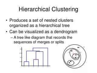
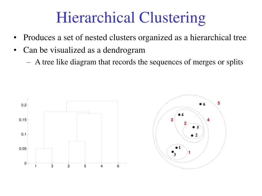
Hierarchical Clustering • Produces a set of nested clusters organized as a hierarchical tree • Can be visualized as a dendrogram • A tree like diagram that records the sequences of merges or splits
Strengths of Hierarchical Clustering • Do not have to assume any particular number of clusters • ‘cut’ the dendogram at the proper level • They may correspond to meaningful taxonomies • Example in biological sciences e.g., • animal kingdom, • phylogeny reconstruction, • …
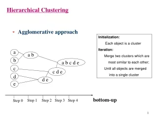
Hierarchical Clustering • Two main types of hierarchical clustering • Agglomerative: • Start with the points as individual clusters • At each step, merge the closest pair of clusters until only one cluster (or k clusters) left • Divisive: • Start with one, all-inclusive cluster • At each step, split a cluster until each cluster contains a point (or there are k clusters) • Traditional hierarchical algorithms use a similarity or distance matrix • Merge or split one cluster at a time
Agglomerative Clustering Algorithm Compute the proximity matrix Let each data point be a cluster Repeat Merge the two closest clusters Update the proximity matrix Until only a single cluster remains • Key operation is the computation of the proximity of two clusters • Different approaches to defining the distance between clusters distinguish the different algorithms
p1 p2 p3 p4 p5 . . . p1 p2 p3 p4 p5 . . . Starting Situation • Start with clusters of individual points and a proximity matrix Proximity Matrix
C1 C2 C3 C4 C5 C1 C2 C3 C4 C5 Intermediate Situation • After some merging steps, we have some clusters C3 C4 Proximity Matrix C1 C5 C2
C1 C2 C3 C4 C5 C1 C2 C3 C4 C5 Intermediate Situation • We want to merge the two closest clusters (C2 and C5) and update the proximity matrix. C3 C4 Proximity Matrix C1 C5 C2
After Merging • The question is “How do we update the proximity matrix?” C2 U C5 C1 C3 C4 C1 ? ? ? ? ? C2 U C5 C3 C3 ? C4 ? C4 Proximity Matrix C1 C2 U C5
p1 p2 p3 p4 p5 . . . p1 p2 p3 p4 p5 . . . How to Define Inter-Cluster Similarity Similarity? • MIN • MAX • Group Average Proximity Matrix
p1 p2 p3 p4 p5 . . . p1 p2 p3 p4 p5 . . . How to Define Inter-Cluster Similarity • MIN • MAX • Group Average Proximity Matrix
p1 p2 p3 p4 p5 . . . p1 p2 p3 p4 p5 . . . How to Define Inter-Cluster Similarity • MIN • MAX • Group Average Proximity Matrix
p1 p2 p3 p4 p5 . . . p1 p2 p3 p4 p5 . . . How to Define Inter-Cluster Similarity • MIN • MAX • Group Average Proximity Matrix
Cluster Similarity: MIN • Similarity of two clusters is based on the two most similar (closest) points in the different clusters • Determined by one pair of points
5 1 3 5 2 1 2 3 6 4 4 Hierarchical Clustering: MIN Nested Clusters Dendrogram
Two Clusters Strength of MIN Original Points Can handle non-globular shapes
Original Points Four clusters Three clusters: The yellow points got wrongly merged with the red ones, as opposed to the green one. Limitations of MIN Sensitive to noise and outliers
Cluster Similarity: MAX • Similarity of two clusters is based on the two least similar (most distant) points in the different clusters • Determined by all pairs of points in the two clusters
4 1 2 5 5 2 3 6 3 1 4 Hierarchical Clustering: MAX Nested Clusters Dendrogram
Original Points Four clusters Three clusters: The yellow points get now merged with the green one. Strengths of MAX Less susceptible respect to noise and outliers
Two Clusters Limitations of MAX Original Points Tends to break large clusters
Cluster Similarity: Group Average • Proximity of two clusters is the average of pairwise proximity between points in the two clusters.
5 4 1 2 5 2 3 6 1 4 3 Hierarchical Clustering: Group Average Nested Clusters Dendrogram
Hierarchical Clustering: Time and Space • O(N2) space since it uses the proximity matrix. • N is the number of points. • O(N3) time in many cases • There are N steps and at each step the size, N2, proximity matrix must be updated and searched • Complexity can be reduced to O(N2 log(N) ) time for some approaches
MST: Divisive Hierarchical Clustering Build MST (Minimum Spanning Tree) • Start with a tree that consists of any point • In successive steps, look for the closest pair of points (p, q) such that one point (p) is in the current tree but the other (q) is not • Add q to the tree and put an edge between p and q
MST: Divisive Hierarchical Clustering • Use MST for constructing hierarchy of clusters
DBSCAN DBSCAN is a density-based algorithm. Locates regions of high density that are separated from one another by regions of low density. • Density = number of points within a specified radius (Eps) • A point is a core point if it has more than a specified number of points (MinPts) within Eps • These are points that are at the interior of a cluster • A border point has fewer than MinPts within Eps, but is in the neighborhood of a core point • A noise point is any point that is neither a core point nor a border point.
DBSCAN Algorithm • Any two core points that are close enough---within a distance Eps of one another---are put in the same cluster. • Likewise, any border point that is close enough to a core point is put in the same cluster as the core point. • Ties may need to be resolved if a border point is close to core points from different clusters. • Noise points are discarded.
DBSCAN: Core, Border and Noise Points Original Points Point types: core, border and noise Eps = 10, MinPts = 4
Clusters When DBSCAN Works Well Original Points • Resistant to Noise • Can handle clusters of different shapes and sizes
When DBSCAN Does NOT Work Well Why DBSCAN doesn’t work well here?
DBSCAN: Determining EPS and MinPts • Look at the behavior of the distance from a point to its k-th nearest neighbor, called the kdist. • For points that belong to some cluster, the value of kdist will be small [if k is not larger than the cluster size]. • However, for points that are not in a cluster, such as noise points, the kdist will be relatively large. • So, if we compute the kdist for all the data points for some k, sort them in increasing order, and then plot the sorted values, we expect to see a sharp change at the value of kdist that corresponds to a suitable value of Eps. • If we select this distance as the Eps parameter and take the value of k as the MinPts parameter, then points for which kdist is less than Eps will be labeled as core points, while other points will be labeled as noise or border points.
DBSCAN: Determining EPS and MinPts • Eps determined in this way depends on k, but does not change dramatically as k changes. • If k is too small ? then even a small number of closely spaced points that are noise or outliers will be incorrectly labeled as clusters. • If k is too large ? then small clusters (of size less than k) are likely to be labeled as noise. • Original DBSCAN used k = 4, which appears to be a reasonable value for most twodimensional data sets.
Fuzzy Clustering • Consider an object that lies near the boundary of two clusters, but is slightly closer to one of them. • In many such cases, it might be more appropriate to assign a weight wij to each object xi and each cluster Cj that indicates the degree to which the object belongs to the cluster Cj. • Fuzzy clustering is based on fuzzy set theory. • Fuzzy set theory allows an object to belong to a set with a degree of membership between 0 and 1, while fuzzy logic allows a statement to be true with a degree of certainty between 0 and 1.
Example • Consider the following example of fuzzy logic. The degree of truth of the statement "It is cloudy" can be defined to be the percentage of cloud cover in the sky, • E.g. if the sky is 50% covered by clouds, then we would assign "It is cloudy" a degree of truth of 0.5. • If we have two sets, "cloudy days" and "non cloudy days," then we can similarly assign each day a degree of membership in the two sets. • Thus, if a day were 25% cloudy, it would have a 25% degree of membership in "cloudy days" and a 75% degree of membership in "non-cloudy days."
Fuzzy Clusters • Set of data points X= {xl,…,xm}, where each point, is an n-dimensional point. • Fuzzy collection C1, C2, ..., Ck • The membership weights (degrees), wij, are assigned values between 0 and 1 for each point, xi, and each cluster, Cj. • We also impose the following reasonable conditions on the clusters: • All the weights for a given point, xi, add up to 1. • Each cluster, Cj, contains, with non-zero weight, at least one point, but does not contain, with a weight of one, all of the points.
Fuzzy c-means algorithm Select an initial fuzzy pseudo-partition, i.e., randomly assign values to all the wij subject to the constraint that the weights for any object must sum up to 1. repeat Compute the centroid of each cluster using the fuzzy pseudo-partition. Recompute the fuzzy pseudo-partition, i.e., the wij. until The centroids don't change.
Computing centroids • Similar to the traditional definition except that all points are considered • Any point can belong to any cluster, at least somewhat. • The contribution of each point to the centroid is weighted by its membership degree. • What happens in the case of traditional crisp sets? • All wij are either 0 or 1, this definition reduces to the traditional definition of a centroid. • Aspgets larger, the partition becomes fuzzier. • p=2 good value.
Updating the Fuzzy Pseudo-partition • This step involves updating the weights wijassociated with the ithpoint and jthcluster. • Intuitively, the weight wij[which indicates the degree of membership of point xi in cluster Cj]should be relatively high if xi is close to centroid cj[if dist(xi,cj)is low] and relatively low if xi is far from centroid cj[if dist(xi,cj)is high]. • If wij = 1/dist(xi, cj) [which is the numerator of equation] then this will indeed be the case. • However, the membership weights for a point will not sum to one unless they are normalized; • i.e., divided by the sum of all the weights aswe do in the equation.
HICAP: Hierarchical Clustering with Pattern Preservation Xiong, Steinbach, Tan, and Kumar 2003
Pattern Preserving Clustering: Motivation • In many domains, there are groups of objects that are involved in strong patterns that are key for understanding the domain. • In text mining, collections of words that form a topic. • In genomics, sequences of nucleotides that form a functional unit. • We want to design a clustering method that preserves these patterns, i.e. that puts the objects supporting these patterns in the same cluster. • Otherwise, the resulting clusters will be harder to understand and interpret. • The value of a data analysis is greatly diminished for end users.
Review: Crosssupport patterns • They are patterns that relate a highfrequency item such as milk to a lowfrequency item such as caviar. • Likely to be spurious because their correlations tend to be weak. • E.g. confidence of {caviar}{milk} is likely to be high, but still the pattern is spurious, since there isn’t probably any correlation between caviar and milk. • Observation: On the other hand, the confidence of {milk}{caviar} is very low. • Crosssupport patterns can be detected and eliminated by examining the lowest confidence rule that can be extracted from a given itemset. • Such confidence should be above certain level for the pattern to not be cross-support one.
Review: Finding lowest confidence • Recall the antimonotone property of confidence: conf( {i1 ,i2}{i3,i4,…,ik} ) conf( {i1 ,i2 ,i3}{i4,…,ik} ) • This property suggests that confidence never increases as we shift more items from the left to the righthand side of an association rule. • Hence, the lowest confidence rule that can be extracted from a frequent itemset contains only one item on its lefthand side.
Review: Finding lowest confidence • Given a frequent itemset {i1,i2,i3,i4,…,ik}, the rule {ij}{i1 ,i2 ,i3, ij-1, ij+1, i4,…,ik} has the lowest confidence if s(ij) = max {s(i1), s(i2),…,s(ik)} • This follows directly from the definition of confidence as the ratio between the rule's support and the support of the rule antecedent.
Review: Finding lowest confidence • Summarizing, the lowest confidence attainable from a frequent itemset {i1,i2,i3,i4,…,ik}, is • This is also known as the h-confidence measure or all-confidence measure. • Crosssupport patterns can be eliminated by ensuring that the hconfidence values for the patterns exceed some user specified threshold hc. • h-confidence is antimonotone, i.e., • hconfidence({i1,i2,…, ik}) hconfidence({i1,i2,…, ik+1 }) • and thus can be incorporated directly into the mining algorithm.
Hyperclique Patterns • An itemset P = {i1, i2, …, im} is a hyperclique pattern if h-confidence(P) > hc, where hc is a user-specified minimum h-confidence threshold. Some hyperclique patterns identified from words of a (news) document collection.
Pattern Preservation? • What happens to hyperclique patterns [sets of objects supporting hyperclique patterns] when data is clustered by standard clustering techniques, e.g., how are they distributed among clusters? • Experimentally found that hypercliques are mostly destroyed by standard clustering techniques. • Reasons • Clustering algorithms have no built-in knowledge of these patterns and have goals that may be in conflict with preserving patterns, • e.g., minimize distance of points from their closest cluster centroid. • Many clustering techniques are not overlapping, i.e. clusters cannot contain the same object (for hierarchical clustering, clusters on the same level cannot contain the same objects). • But, patterns are typically overlapping.
HICAP Algorithm • Find maximal hyperclique patterns • Non-maximal hypercliques will tend to be absorbed by their corresponding maximal hyperclique pattern and not affect the clustering process. • Thus, using all hyperclique patterns would cause a great deal of overhead with little if any gain. • Perform a group average hierarchical clustering • The starting clusters are hyperclique patterns and the points not covered by hyperclique patterns. • Except for the starting point, the clustering algorithm is the same as the group average approach. • Since hypercliques are overlapping, resulting clustering may also be overlapping.