Download
1 / 32
330 likes | 418 Vues
Project Proposal Changes in atmospheric energy transport into Arctic in the greenhouse gas forced future Natasa Skific Department of Atmospheric Sciences Rutgers University.

E N D
Project ProposalChanges in atmospheric energy transport into Arctic in the greenhouse gas forced futureNatasa SkificDepartment of Atmospheric SciencesRutgers University
“The more clearly we can focus our attention on the wonders and realities of the universe, the less taste we shall have for its destruction”… (Rachel Carson).
1000 years of changes in carbon emissions, concentrations and temperature ACIA, 2004
Extended time scale ACIA, 2004 Ruddimann (2003)
Zonally-averaged time series of annual surface temperature anomalies (°C) from 1891-1999 north of 30°N (from Johanessen et al. 2004).
Are there mechanisms within our climate system that can offset the predicted Arctic change? • Most individual climate feedbacks in the Arctic climate system are overwhelmingly positive (Serreze and Barry, 2005, Overpeck et al., 2005). • Are there feedbacks outside the Arctic climate system with the potential to arrest the predicted high-latitude warming?
Schematics of the energy balance for the north polar cap (from Nakamura and Oort, 1988). Fwall is moist static energy flux: F rad 70° 70° ΔE/Δt Fwall Fwall F surf Sensible heat flux Latent heat flux Potential energy flux
Overland et al., 1994. Geopotential Transport + Sensible Transport = “Dry Static Energy Flux” (DSE) Steven Vavrus, personal communications
Relative contributions of components of energy transport to total flux across 70º N for various seasons Winter Summer Overland et al., 1994.
How is the moist static energy flux going to respond to the Arctic change? • If Arctic warming is enhanced in response to increasing greenhouse gas concentrations, the lower-tropospheric poleward temperature gradient should relax, poleward advection of sensible heat should decrease, and Arctic warming should relax (negative feedback). • How will the latent heat flux change? • Will latent heat flux compensate for the reduction in sensible heat flux? • How will the energy flux change at various levels? • Climate models show an increased warming of the tropical upper troposphere, which could increase the sensible heat flux in the upper layers of the troposphere.
Data sets • European Center for Medium Range Forecast Reanalysis (ERA-40), http://data.ecmwf.int/data/d/era40_daily. • The National Center for Atmospheric Research Community Climate System Model, version 3.0, T85 L26 (NCAR CCSM3), http://www.cgd.ucar.edu/ccr/strandwg/. • The 21st century simulation incorporates the Special Report on Emission Scenario (SRES) A2 scenario [Nakicemovic and Swart, 2000], or the “worst case scenario” (probably the most likely to occur, [Rahmstorf et al., 2007]).
SRES A2 Arctic surface temperature change, °C. “emerging state” warming “mature state” warming Mean surface temperature, 2011-2030 minus 1980-1999. Mean surface temperature, 2070-2089 minus 1980-1999.
Self-organizing map approach • Self-organizing maps (SOMs) are a data visualization technique (T. Kohonen, 1995), which uses unsupervised learning algorithm to reduce the dimensions of large data sets by grouping similar data sets together, organizing them into a two-dimensional array or a map. • SOMs accomplish 2 goals: • a.) reduce dimensions • b.) display similarities • Steps of the SOM routine: • 1.) creation of a first guess map • 2.) map training (data sample is presented to the SOM, similarity between the data and each reference vector is calculated as a measure of Euclidean distance in space, “best match” node is found and the reference vectors are modified so that • hci is a neighborhood function
Frequency of occurrence (%) of each individual node of sea-level pressure (right) compared to an even distribution (left). 1025 hPa Thickness of each box is the number of samples from the original dataset matching to a particular node. Control Sample 1000 hPa Colors of each box show mean sea-level pressure for each node north of 70°N
Mapping meridional moisture flux of ERA-40, kg/(ms), across 70°N onto the SLP field.
Mapping total moisture flux convergence (cm/mo) by ERA-40 onto the SLP field. Example: Moisture convergence pattern for low pressure above the Barents Sea.
SOM for winter (DJF) tropospheric convergence of sensible heat, 1979-2002, ERA-40. Projections of reference vectors in 2-dim space for various stages of map training (Kohonen, 1990). t=20 t=1000 t=5000 t=100000 Sammon mapping applied to SOM (above), showing the local relationship between the nodes in a two-dimensional space. Example: Projection of node 35 on a 2-dim space.
Moisture fluxes for ERA-40, winter (NDJFM) in kg/(ms) Moisture fluxes for ERA-40, summer (MJJAS) in kg/(ms) Zonal flux Meridional flux
Seasonal means for moisture convergence, ERA-40, cm/mo, 1000-300 hPa
Moisture convergence, ERA-40, (left) and CCSM3(right), 1958-1999 mean layer 1000-300 hPa, units: cm/mo ERA-40 NCAR CCSM3
What remains to be done: • Calculate the remaining fluxes (sensible energy and potential energy flux) using NCAR-CCSM3, for 20th and 21st century. • Apply the SOM technique of moist static energy to investigate its spatial and temporal variability and predict future behavior. • Investigate model’s realism of performance for the 20th century by using ERA-40. • Correlate horizontal transports with large-scale circulation patterns, such as the NAO/AO. • Map variables of energy transport onto a sea-level pressure SOM of NCAR’s CCSM3 to explore how spatial patterns change for a particular circulation regime. • Publish results !!! We hope to contribute to understanding of the role of energy transport into Arctic and its potential to arrest the predicted Arctic change.
Trends (°C/decade) in Arctic surface temperature by season from 1981-2005 based on clear-sky Advanced Very High Resolution Radiometer (AVHRR) retrievals (updated from Comiso, 2003, using improved retrieval algorithms).
Arctic Amplification winter summer
Each term in equation can be expanded into three components: Transient eddies Stationary eddies Mean meridional circulation Overland et al., 1994.
Data sets (cont). • NCAR CCSM3 20th century run spans time period of 1950-1999, 20C3M. • The 20th century experiment (20C3M) includes: • forcing by the observed concentrations of CO2, CH4, N2O and CFCs; • ozone forcing [Kiehl et al., 1999]; • solar forcing [Lean et al., 2002]; • Parameterization of the effects of volcanic eruptions [Ammann et al., 2003]; • direct effect of sulfates [Smith et al., 2001, 2004a], with no indirect aerosol forcing included.
Data sets (cont). • The 21st century simulation incorporates the Special Report on Emission Scenario (SRES) A2 scenario [Nakicemovic and Swart, 2000], or the “worst case scenario” (probably the most likely to occur, [Rahmstorf et al., 2007]), which assumes continuously increasing population (15 billion by the year 2100), and slow implementation of new technologies. “emerging greenhouse state” “mature greenhouse state”
Arctic Oscillation Positive AO Negative AO Regression of winter DJF AO index onto surface air temperature 1960-2000, NCAR CCSM3 Leading eof of the winter (DJF) sea-level pressure, NCAR CCSM3
SOM for winter (DJF) tropospheric sensible heating, 1979-2002, ERA-40. Difference of the frequency of occurrence for days with the high AO minus days with the low AO index. Sammon mapping applied to SOM (above), showing the local relationship between the nodes in a two-dimensional space.
Moisture fluxes for ERA-40, winter (NDJFM) in kg/(ms) Moisture fluxes for ERA-40, summer (MJJAS) in kg/(ms) Zonal flux Meridional flux