Download

1 / 52

E N D
HEAT PROCESSES HP7 Heat exchangers thermal design Shell and tube HE. Comparison 1-1 and 1-2 arrangements from point of view of pressure drops and heat transfer. Enthalpy balance of HE, temperature profiles, effectiveness, LMTD, sizing and rating design methods. NTU-epsilon method for parallel flows (eigenvalue problem, derived temperature profiles and eps), counter current and cross flow arrangement of streams (sheet of selected NTU-eps correlations from Rohsenow). Asymptotical properties. Zonal method. Graphical design (Roetzel Spang diagrams from VDI). Rudolf Žitný, Ústav procesní a zpracovatelské techniky ČVUT FS 2010
HEAT EXCHANGERS HP7 Heat exchangers Recuperative Regenerative Rotating drum Wall separating streams Direct contact
HEAT EXCHANGERS HP7 Compactness Hydraulic diameter, mm 10 1 0.1 60 lungs Special Car cooler Plate and fin Plate Shell-&-tube 1000 10 000 100 m2/m3
HE Shell & Tube HP7 Shell&Tube are the most frequently used and universal heat exchangers Tanguy
HE Shell & Tube HP7 • 300 bar shell, 1400 bar pipe • -100 up to 600oC • For any media • Maximal effectivnesse = 0.9 • MinimalDT = 5 K • 10 up to 1000 m2 Terminology STHE Example cpndenser 1-2 (one pass in shell, two passes in tubes) ROD baffles Segmental baffles ) ABB Lummus Helical baffles
L(=A) M(=B) N A E 1pass F 2passes B T G C S H N P J D X W HE Shell & Tube TEMA HP7 TEMA (Tubular Exchanger Manufact. Assoc.) specification FRONT HEAD SHELL REAR HEAD Front head design depends upon pressures, cleaning requirements etc Floating rear heads are necessary in case of large temperature differences (dilatation)
HE Shell & Tube TEMA HP7 TEMA (hydraulic & thermal design based upon Delaware method) A-leakage through gap tube-baffle Wolverine Engineering Data Book II. (Wolverine Tube Inc. 2001) B-cross flow C-bypass outside bundle Idea: basic correlations for the friction factor f and the heat transfer coefficient are corrected by factors reflecting parallel streams A,B… E-leakage through gap shell-baffle J-faktor (Colburn)
L L HE Shell & Tube HP7 Example: Comparison 1-1 and 1-2 (for the same dimensions, number of tubes, flowrate...) With 2 passes in tubes the mean velocity increased 2x, path increased 2x, heat transfer surface the same. Therefore pressure drop will be increased 4x in laminar and 8x in fully developed turbulent regime (Fanning factor f is indirectly proportional to velocity in laminar, while f is constant in turbulent regime). On the other hand increased velocity in the 2pass configuration decreases fouling rate and increases heat transfer. Nusselt number is Re1/3 and Re0.8 in laminar and turbulent regime, respectively. Therefore heat transfer coefficient increases 21/3=1.26 times in laminar, and 20.8=1.7 times in turbulent flow regime.
HE Plate HP7 Plate & Frame heat exchanger Chevron corrugated plate Welded plate HE
HE Plate-Fin ALPEMA standard HP7 ALPEMA THE STANDARDS OF THE BRAZED ALUMINIUM PLATE-FIN HEAT EXCHANGER MANUFACTURERS' ASSOCIATION Terminology Plate-Fin HE
HE Thermal design HP7 Tanguy
HE Thermal design HP7 SIZING methods (how to calculate heat transfer surface, given temperatures and flow rate) RATING methods (how to calculate outlet temperatures and duty for given HE) Thermal design is based upon enthalpy balances and upon calculation of temperature profiles using correlations for heat transfer coefficients. Results are frequently expressed in form of design diagrams. Alternative approach is CFD (Computer Fluid Dynamics)
W2 T2’ Q=kST W2 T2’’ W1 T1’ Qloss W1 T1’’ HE Thermal design HP7 Capacity rate W [W/K] is calculated for one phase flow as Enthalpy balance of the whole HE (steady state) Enthalpy balance of the stream 1 (steady state) There are three unknowns when RATING: outlet temperatures and Q (duty of HE). Heat losses Qloss are usually small and can be neglected or estimated knowing thermal resistance of insulation. There is only one unknown when SIZING: “effective” heat transfer surface kS .
HE Thermal design HP7 Enthalpy balances represents only 2 equations, the third one is where k is overall heat transfer coefficient calculated from heat transfer coefficients on both streams, thermal resistance of fouling layers and thermal resistance of wall (thickness h) Mean temperature difference is defined as Mean temperature difference can be calculated only if detailed temperature profiles inside HE are known (see later).
T1’ T1’ T1 T1 T1’’ T1’’ ’=T1’-T2’ ’=T1’-T2’ =T1-T2 =T1-T2 ’’=T1’’-T2’’ ’’=T1’’-T2’’ T2’’ T2’’ T2 T2 T2’ T2’ Qs s Q S HE Thermal design HP7 Only in the case of two parallel flows it is possible to calculate the mean temperature difference as LMTD (logarithmic mean temperature difference) This diagram was used in PINCH analysis. Do you remember? (composite curves of hot and cold streams)
T1’ T1 T1’’ ’=T1’-T2’ =T1-T2 ’’=T1’’-T2’’ T2’’ T2 T2’ Qs Q HE Thermal design HP7 Proof follows from the linear relationship between temperature and enthalpy flow Qs and this is ordinary differential equation which can be integrated giving
T1’ T1 ’=T1’-T2’’ T1’’ =T1-T2 T2’’ ’’=T1’’-T2’ T2 T2’ Qs Q HE Thermal design HP7 The same holds for the counter current heat exchanger = proof is identical etc., with the same result:
HE Thermal design HP7 This approach cannot be used for more complicated arrangement of streams, for example cross-flow HE (temperature distribution in streams are functions of two variables x,y). Even the HE with parallel flows with more than one pass or more than two streams must be based upon temperature profiles expressed as functions of coordinates (x,y, or heat transfes surface measured from one end of HE). In this case temperature profiles are calculated from enthalpic balances of individual streams (or individual passes). For example the previous case of two parallel flows is solved from two balances (x-distance from one end of HE) Enthalpy balances x (k is heat transfer coef. related to unit length of HE!! not to the unit heat transfer surface, check units)
HE Thermal design HP7 These differential equations can be written in matrix form This system of coupled differential equations is transformed to uncoupled system by transformation (temperatures T(x) are transformed to new variables Z(x)) where U is eigenvector matrix associated to conductivity matrixA where is diagonal matrix of eigenvalues 1 2. To find out eigenvector matrix and eigenvalues given matrix A is standard operation available in scientific computer libraries, for example using single command in MATLAB[L,U]=eig(A).
HE Thermal design HP7 Substituting the transformation to diff. equations results the uncoupled system Uncoupled because [[]] is a diagonal matrix solution Coefficients d1, d2 are determined by boundary conditions (end temperatures).
æ ö 0 0 æ ö 1 W ç ÷ ç ÷ 2 = L = 1 1 [[ U ]] [[ ]] ç ÷ ç ÷ - + 0 k ( ) - 1 W ç ÷ è ø W W 1 è ø 1 2 æ ö æ ö æ ö T ' 1 W d + - W T ' W T ' T ' T ' ç ÷ ç ÷ ç ÷ 1 2 1 = = = d 1 1 2 2 d 1 2 ç ÷ ç ÷ ç ÷ 1 2 - + + T ' 1 W d W W W W è ø è ø è ø 2 1 2 1 2 1 2 1 l = + + - L T ' ' ( W T ' W T ' ( T ' T ' ) W e ) 2 1 1 1 2 2 1 2 2 + W W 1 2 1 l = + - - L T ' ' ( W T ' W T ' ( T ' T ' ) W e ) 2 2 1 1 2 2 1 2 1 + W W 1 2 HE Thermal design HP7 Special case of two streams can be solved analytically and easily, because eigenvalue prob lem has the solution (verify) therefore boundary conditions at x=0 giving . Temperatures at outlet (x=L, length of HE) are therefore x L
recommended for reading HE Thermal designpaper Roetzel HP7 Xing Luo, Meiling Li, Wilfried Roetzel: A general solution for one-dimensional multistream heatexchangers and their networks. International Journal of Heat and Mass Transfer 45 (2002) 2695–2705 This paper describes the previous method of temperature profiles calculation in more details. It is always usefull to read Roetzel’s papers A mathematical model for predicting the steady-state thermal performance of one-dimensional (cocurrent andcountercurrent) multistream heat exchangers and their networks is developed and is solved analytically for constantphysical properties of streams. By introducing three matching matrices, the general solution can be applied to varioustypes of one-dimensional multistream heat exchangers such as shell-and-tube heat exchangers, plate heat exchangersand plate–fin heat exchangers as well as their networks. The general solution is applied to the calculation and design ofmultistream heat exchangers. Examples are given to illustrate the procedures in detail. Based on this solution thesuperstructuremodel is developed for synthesis of heat exchanger networks. Thermal flow rate U=kS/L Vector D is determined by boundary conditions (temperatures) Eigenvectors of A Eigenvalues
HE Thermal designpaper Roetzel HP7 Analytical expression for temperature profiles in subchannels Coefficients[d] follow from boundary conditions (inlet temperatures at N streams) and from the fact that outlet temperatures of M- subchannels are inlet temperatures of connected subchannels (defined by matrix[[G]]). Inlet temperatures of subchannels are either inlet temperatures of streams or outlet temperatures of connected subchannels This is system of M linear algebraic equations for vector [d]. Outlet temperatures can be expressed as
+ W W kL W l = = = + = + L E e exp(-kL ) exp(- ( 1 )) exp(-NTU ( 1 W )) 1 2 1 2 W W W W 1 2 1 2 kL kS = = NTU NTU W W 1 1 1 l = + + - L T ' ' ( W T ' W T ' ( T ' T ' ) W e ) 2 1 1 1 2 2 1 2 2 + W W 1 2 HE Thermal design HP7 Please return back to the previously derived expressions for outlet temperatures The exponential term can be expressed in terms of two dimensionless parameters, that play important role in thermal design of HE The fist criterion NTU (Number of Transfer Units) is a measure of HE size (usually defined as with the overall heat transfer coefficient k related to unit heat transfer surface) The second parameter W is ratio of heat capacities of streams (thermal flow rates Wi).
T1’ W1<W2 T2’’ - - Q W ( T ' T ' ' ) T ' T ' ' T1’’ e = = = 1 1 1 1 1 - - Q W ( T ' T ' ) T ' T ' T2’ max 1 1 2 1 2 HE Thermal design HP7 e The third criterion (characteristics) of HE is effectiveness defined as an actual duty of HE to the duty of ideal HE (infinite heat transfer surface S, countercurrent flow orientation) at the same flow rates and thesame inlet temperatures, therefore The interpretation that the temperature ratio (temperature drop of the first stream)/(difference of inlet temperatures) is the ratio of actual power (duty) to the maximum power transferred by an ideal heat exchanger with infinite heat transfer surface is correct only if the stream 1 is weaker, because only than the temperature of the weaker stream can approach to the inlet temperature of the stream 2. Temperature profile for the actual HE Temperature profile for the HE with infinite heat transfer surface
e Asymptot ic behaviour for NTU<<1 NTU= - Q kS ( T ' T ' ) e = = = NTU 1 2 - Q W ( T ' T ' ) max 1 1 2 HE Thermal design HP7 What does it mean? For small HE (small heat transfer surface related to heat capacity W) you need not worry about a specific relationship =f(NTU,W). All small HE are the same. Balthus
HE Thermal design zonal method HP7 e The fact that for small HE holds NTU= is the basis of numerical ZONAL methods (HE is substituted by a network of small HE and system of internal temperatures is solved iteratively). T2’ W2 T1’ W1 zone NTUzone T1’’=T1’-zone(T1’-T2’) T2’’=T2’+W1/W2zone(T1’-T2’)
= - Q W ( T ' T ' ' ) 1 1 1 Q = kS D T HE Thermal design HP7 Summary of thermal design methods RATING methods SIZING methods given Temperatures and flowrates given Size (S) and inlet temperatures calculated S calculated outlet temperatures and Q e calculate from NTU and W. e calculate one output temperature T ’ from 1 and second outlet temperature from the enthalpy balance.
HE design diagrams HP7 Banks
HE design diagrams F-correction HP7 Method LMTD, Bowman et al. (1940) is an example of SIZING methods. Heat transfer surface is calculated from where TLM is logarithmic mean temperature difference (LMTD) based only upon inlet and outlet temperatures (see next). FT is a correction factor dependent upon and W. Remark: HEDH (Heat Exchanger Design Handbook) use the symbol P for thermal effectiveness (instead of ) and the symbol R as the ratio of heat capacities (instead of W, shown in the graph) FT<0.75 indicates unsuitable flow arrangement (use a different configuration of HE)
T1’ T1 ’=T1’-T2’’ T1’’ =T1-T2 T2’’ ’’=T1’’-T2’ T2 T2’ HE design diagrams F-correction HP7 Logarithmic Mean Temperature Difference is expressed only by inlet/outlet temperatures of both streams, not taking into account specific location of inlet/outlet ports. The following definition is quite general This LMTD corresponds to the counter-current heat exchanger. For any other (nonideal) HE it is necessary to decrease the TLM value by the F-correction
T1’ T1’ W1<W2 T1’’ T2’’ T2’’ T1’’ W1>W2 T2’ T2’ HE design diagrams F-correction HP7 The correctionTLMdepends upon two parameters As soon as the stream2is weaker (W1>W2, R<1) the parameter P can be called effectiveness (and denoted by symbol ). Effectiveness is the ratio of thermal power Q of the analysed exchanger to the power Qmax of an ideal (counter current) HE having infinite heat transfer surface. In that case outlet temperature of the stream 2 approaches inlet temperature of the stream 1 (T1’=T2’’)
HE design diagrams F-correction HP7 Examples F-correction diagrams from Kakac S. Boilers, Evaporators and condensers, Wiley 1991
1 HE design diagrams F-correction 2 HP7 F-correction of LMTD R For shell & tube heat exchangers with 2 passes in pipes T1-temperatures in shell, T2-temperatures in pipes
HE design diagrams F-correction (Example) HP7 F-correction LMTD Temperature crossing B A T1’ T1’ T1’’ T2’’ T2’’ PB PA T1’’ FTA T2’ T2’ The variants A,B of the same heat exchanger differ only by reverting flow direction in shell.The variant B isIRRONEOUS with a possible temperature crossing. However effectiveness P and the FT values are the same.
HE design diagrams F-correction (Example) HP7 The exchanger can be calculated by MATLAB using zonal method B for iter=1:30 for i=1:n-1 a=(t1(i)+t1(i+1))/2; t2a(i+1)=a+(t2a(i)-a)*e2; end t2b(n)=t2a(n); for i=n-1:-1:1 a=(t1(i)+t1(i+1))/2; t2b(i)=a+(t2b(i+1)-a)*e2; end for i=n-1:-1:1 a=(t2a(i)+t2a(i+1)+t2b(i)+t2b(i+1))/4; t1(i)=a+(t1(i+1)-a)*e1; end end l=1; length L=1 m w1=1; heat capacity of stream 1 (shell) w2=1; heat capacity of stream 2 (pipes) ks=1; kS-the heat transfer surface (1 pass) t1in=100; inlet temperature shell t2in=10; inlet temperature tubes n=500; dz=l/(n-1); t1(1:n)=t1in; t2a(1:n)=t2in; t2b(1:n)=t2in; e1=exp(-2*ks*dz/w1); NTU-stream shell e2=exp(-ks*dz/w2); NTU-stream pipes A B
HE design diagrams F-correction (Example) HP7 NTU1=kS/W1- tubes, NTU2=kS/W2 - shell Exactly the same problem can be solved by the following excel program You should specify inlet temperatures at tubes (blue stream) and shell (read stream)
HE design diagrams F-correction (Example) HP7 The previous Excel program compares the zonal method with the approximation based upon assumption that the shell stream can be divided into two streams exchanging heat with the tube streams and only at the exit these two streams are mixed. Specify inlet temperature and heat capacity of the shell stream Specify kS for the first and the second pass Specify kS for the first and the second pass Specify outlet tube temperature
HE design diagrams F-correction (Example) HP7 • When comparing the Excel and MATLAB solution you see that: • MATLAB solution is clear and readable • MATLAB solution enables to use variable number of zones easily EXCEL programming is a hell nicely described by Hieronimus Bosch
HEAT EXCHANGERS design diagrams HP7 Unlike the Bowman’s F-correction the Kays London (1964) NTU-eps method is suitable for RATING. Given the heat transfer surface (NTU) and capacities of stream W it is possible to read effectiveness from appropriate graphs and
HEAT EXCHANGERS design diagrams HP7 Roetzel Spang diagrams (1990) see VDI Warmeatlas
R1 NTU1 P1 R2 NTU2 P2 HEAT EXCHANGERS design diagrams HP7 Roetzel Spang diagrams (1990) see VDI Warmeatlas R1 Red line NTU P1 R2 NTU1 NTU2 P2 Small HE (NTU<0.1) are really the same R1 NTU1 P1 R2 Not only the counter-current HE but also some kinds of cross-flow HE are capable to achieve P=1 at arbitrary R NTU2 P2 R1 NTU1 P1 R2 Asymmetry of NTU curves indicates, that effectiveness depends upon exchange of streams NTU2 P2
HE CFD analysis selected papers HP7 Computer Fluid Dynamics analysis yields interesting data important for structural, fouling and RTD analysis, identification of flow irregularities, dead spaces, shortcuts, etc… However, accuracy of heat transfer and pressure drop prediction is seldom better than 10%. Results hold usually only to a specific design and dimensions. Miro
HE CFD analysis papers (segmental baffles) HP7 Ender Ozden, Ilker Tari: Shell side CFD analysis of a small shell-and-tube heat exchanger. Energy Conversion and Management 51 (2010) 1004–1014 The shell side design of a shell-and-tube heat exchanger; in particular the baffle spacing, baffle cut and shell diameter dependencies of the heat transfer coefficient and the pressure drop are investigated by numerically modeling a small heat exchanger. The flow and temperature fields inside the shell are resolved using a commercial CFD package. A set of CFD simulations is performed for a single shell and single tube pass heat exchanger with a variable number of baffles and turbulent flow. The results are observed to be sensitive to the turbulence model selection. The best turbulence model among the ones considered is determined by comparing the CFD results of heat transfer coefficient, outlet temperature and pressure drop with the Bell–Delaware method results. For two baffle cut values, the effect of the baffle spacing to shell diameter ratio on the heat exchanger performance is investigated by varying flow rate. Too small baffle cut and too long spacing optimum Bell–Delaware recommended segmental baffle cut values as a function of B/Ds ratio. SBC: segmental baffle cuts in no-phase-change flow; CV: baffle cuts applicable to condensing vapors
HE CFD analysis papers (segmental baffles) HP7 Ender Ozden, Ilker Tari: Shell side CFD analysis of a small shell-and-tube heat exchanger. Energy Conversion and Management 51 (2010) 1004–1014
PT Lb HE CFD analysis papers (ROD baffles) HP7 Q.W. Dong, Y.Q. Wang, M.S. Liu: Numerical and experimental investigation of shellside characteristics for RODbaffle heat exchanger. Applied Thermal Engineering 28 (2008) 651–660 RODbaffle heat exchanger is a kind of shell-and-tube heat exchanger with eminent performance. Because of the characteristics of tube bundle support structure, fluid flow on shellside is longitudinal and periodical, and fluid flow is of symmetry in landscape orientation. According to the fluid flow characteristics on shellside and ignoring the impact of inlet, outlet and shell wall, a periodic flow unit duct was taken as the simplified model of the shellside to perform numerical simulation by using CFD code, FLUENT. It was found that the both errors in magnitude of the main fluid velocities and heat transfer coefficients between results of simulation and that of experiment or correlations are less than 10%, and the errors of pressure drop between simulation and correlation are no more than 20%. The detailed characteristics and relation of fluid flow and heat transfer on shellside of the RODbaffle heat exchanger were analyzed using the simulation results. Geometric model of periodic flow unit duct model Correlation used by Philips Petroleum
HE CFD analysis papers (helical baffles) HP7 Jian-Fei Zhang, Ya-Ling He, Wen-Quan Tao: 3D numerical simulation on shell-and-tube heat exchangers with middle-overlapped helical baffles and continuous baffles – Part II: Simulation results of periodic model and comparison between continuous and noncontinuous helical baffles. International Journal of Heat and Mass Transfer 52 (2009) 5381–5389 In this paper, based on the simplified periodic model the performance predictions for heat exchanger with middle-overlapped helical baffles are carried out by 3D simulation for three different helix angles (30, 40and 50), and the commercial codes of GAMBIT 2.3 and FLEUNT 6.3 are adopted in the simulation. It is found that the model average heat transfer coefficient per unit pressure drop of the 40angle case is the largest, which is in qualitative agreement with the existing literature. The predicted average intersection angle of this case is the smallest, being consistent with the field synergy principle. The performance of periodic model with continuous helical baffle is also compared with that of the noncontinuous middle-overlapped helical baffles. It is found that the heat transfer coefficient per unit pressure drop of the noncontinuous middle-overlapped helical baffles is appreciably larger than that of the continuous helical baffle, indicating that the heat exchanger with noncontinuous middle-overlapped helical baffles has its advantage over the one with continuous helical baffle.
EXAM HP7 Heat exchangers Thermal design