Download
1 / 33
330 likes | 489 Vues
Looking for Climate Signals in Ice Cores Santa Fe, 2011. Gerald R. North Thanks to Petr Chylek for the data and encouragement. g-north@tamu.edu. Two simulated time series of length of the time series: N=1000. Pure white noise N(0, 1). Pure white noise N(0, 1) + 0.3 Sin[2 p t/11].

E N D
Looking for Climate Signals in Ice CoresSanta Fe, 2011 Gerald R. North Thanks to PetrChylek for the data and encouragement. g-north@tamu.edu
Two simulated time series of length of the time series: N=1000 Pure white noise N(0, 1) Pure white noise N(0, 1) + 0.3 Sin[2pt/11] This time series has a signal of amplitude 0.3 and period of 11y period added: can you see it?
Pure white noise N(0, 1) + 0.3 Sin[2pt/11] Periodogram: Square of the Discrete Fourier Transform. 10.82y 10.82y Note: 9 out of 500 lines (2.2%) exceed 2 std 2 std above mean We can reduce sampling noise by smoothing the periodogram
Pure white noise N(0, 1) + 0.3 Sin[2pt/11] Here is a 25 line (box car) moving average of the periodogram. Error bar is divided by 5. Note the bias in frequency of the line 12.5y 12.5y
Pure white noise N(0, 1) + 0.3 Sin[2pt/11] Another way: Sort the periodogram into bins with 25 lines in each: 11y peak disappears!
A better approach: Usethe lag window method 0 0 time This step to 0 is too abrupt To reduce the effects of the sharp transition at the beginning and end of the time series we apply the window by: Parzen’s Lag Window
Pure white noise N(0, 1) + 0.3 Sin[2pt/11] 10.83y 10.83y 2 std above mean
Pure white noise N(0, 1) + 0.3 Sin[2pt/11] Example: white noise (s=1) with a sharp peak of amplitude 0.3 at period 11 y Moral: Lag Window (Parzen’s here) is good for sharp lines + noise
Sun Spots and Total Solar Irradiance Amplitude of the 11y oscillation in TSI: 0.07%
Plausibility of seeing the 11y cycle in surface temperature data Estimated Response to 10y Cycle 0.1% TSI Forcing based on a simple energy balance climate model with a slab (mixed layer) ocean (North, Stevens, Wu, 2004)
Simultaneous detection of solar cycle, volcanic, aerosol, greenhouse gases 90% confidence intervals 20 tropical sites 36 global sites Noise-forced North, G. R. and Q. Wu, 2001: Detecting climate signals using space-time EOFs. J. Climate, 14, 1839-1862.
Top-Down influence of the solar cycle on temperatures. Coughlin & Tung, 2004. They used Empirical Mode Decomposition Comment: this effect adds to the surface effect (EBM).
Here is a simulation of white noise background (0, 1) with a 0.05 amplitude sine wave. The white noise is about the variance from year to year in South Greenland. This shows that it is plausible to detect a signal of this strength. The result is robust; I did the simulation many times. The other peaks jump around, but the 11y peak stays relatively fixed. 10.7y
Dye3 Core Results Comments: the Dye 3 site is close to the coast and should reflect AMO, NAO and other activities. But we might look for the 11y cycle as well. The data are 18O which probably indicates temperature at the time of deposition. But it may indicate other things such as North American storm tracks, etc. Dye3
Dye 3 Spectral Density. Conceptual Model: the time series is an AR1 process with possible additive sharp lines. Parzen Window Ideal AR1 spectral density To get the period of oscillation, divide the abscissa into 3600
Dye 3 (South Greenland) analysis for N=3600 years, using the Parzen Window 14.2 10.3 42.1 19.6 95% if freq is known a priori 20 bandwidths (expect 1 peak to exceed --- in 20 BWs)
14C 14C Delaygue&Bard, 2011 10Be 10Be Band-Passed Taylor Dome Time Series Sunspots From Foukal’s book, attributed to Eddy I have no great confidence in my Dye 3 reconstruction (sampling error issues).
Taylor Dome Data personally communicated by PetrChylek Taylor Dome: 600 yr Record http://nsidc.org/data/docs/agdc/nsidc0108_wahlen/index.html
Taylor Dome (Antarctica) analysis for N=600 years, using the Parzen Window 20.0 10.3 5 bandwidths (expect 1 peak to exceed --- in 20 BWs)
Robert G. Currie Papers Currie uses Max Entropy Spectral Analysis to detect the Lunar Tidal (18.6y) and Solar Cycle Peaks in North America Station (and other) data. He pools hundreds of records to increase signal to noise.
The M2 (18.6y) tidal constituent. Amplitude is indicated by color, and the white lines are co-tidal differing by 1 hr. The curved arcs around the amphidromic points show the direction of the tides, each indicating a synchronized 6 hour period.
Thoughts: Surely the solar cycle and the tidal contributions are tiny perturbations in the time series. How could these be important in the spectral analysis? Answer: the tidal 18.6y signal is common to all station time series and coherent (deterministic, nearly same phase at all sites). When we add thousands of records together to form an average, most of the natural variability cancels out, but not the coherent signal. Could this explain the 18 year cycle in the Berkeley record for the 1800s? The tides are big where BEST has data. Answer: the 10.5y signal is from a single time series but the record is 60 cycles long (Taylor Dome) and 360 cycles long (Dye 3) A deterministic peak in a periodogram grows as the record grows, but the noise does not.
Conclusions • Response to 10.5y solar cycle and surface temperature appears to be real. • Surface response appears to be larger than EBM simulation (probable top-down contribution) • There could be a tidal signal (18.6y) in the data. • There is not much evidence for a long term AMO (pure tone at 60 or 70y) in this study.
First Notice of AMO Nature 1994 global average actually named AMO by Richard Kerr, Science
N=3600y Dye 3 Bartlett Window
N=3600y Dye 3 Parzen Window 10.5y
Taylor Dome Bartlett Window
Taylor Dome Parzen Windows