Download
1 / 17
170 likes | 287 Vues
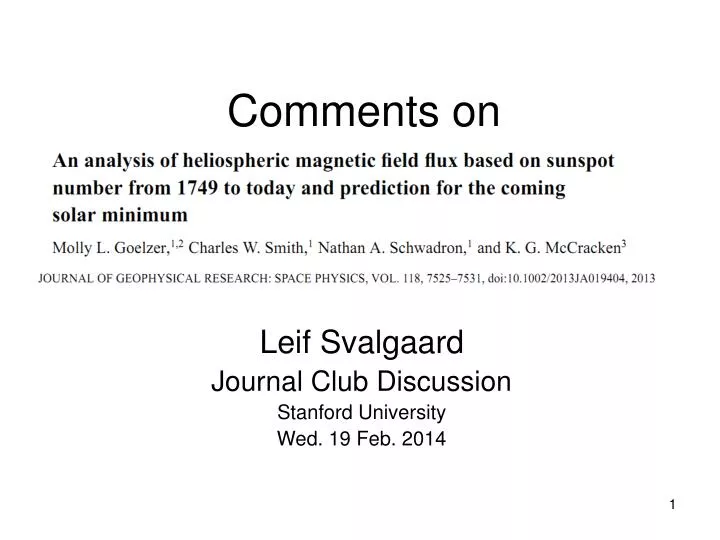
Comments on. Leif Svalgaard Journal Club Discussion Stanford University Wed. 19 Feb. 2014. Magnetic Flux Balance in the Heliosphere Schwadron et al. ApJ 722, L132, 2010. Closed loop CMEs connecting with polar flux reduces the latter, moving it to lower latitudes.

E N D
Comments on Leif Svalgaard Journal Club Discussion Stanford University Wed. 19 Feb. 2014
Magnetic Flux Balance in the Heliosphere Schwadron et al. ApJ 722, L132, 2010 Closed loop CMEs connecting with polar flux reduces the latter, moving it to lower latitudes CMEs eject loops that open up and increase the HMF flux and increase polar holes Disconnection leads to removal of HMF flux and shrinkage of polar holes
The CME Flux Rate The theory posits two components of the HMF: the CME associated magnetic flux xxxx from the ejecta and the open magnetic flux xx of the steady solar wind. The time derivative of the CME-associated flux xx is written as A large fraction, D ≈ ½, of this flux opens as the CME launches from the Sun, so the closed flux created by an individual CME is (1 − D) . The other factor that enters the source term for closed ejecta-associated flux is the frequency, f (t), of CME ejection, which depends on time, t, varying typically from 0.5 day−1 near solar minimum to 3 day−1 near solar maximum. The loss term has three parts: A decay of due to interchange reconnection on a characteristic timescale of ; disconnection on a timescale of ; and opening of the flux loops when they merge into the background on a timescale of . All of there timescales are poorly known, but one can make guesses: xx = 20d, yy = 6y, zz = 2.5y.
The Open Flux Rate For the magnetic flux not associated with CMEs [the ‘open’ flux ] they set the time derivative equal to the loss by disconnection (on timescale xx) subtracted from the source due to the opening of CME-associated flux (on timescale xx), thus: If there is a ‘floor’ on which the CME-associated flux ‘rides’ then the disconnection loss-term should be measured relative to the floor Adding the rate of change of the CME-associated flux, given by And using = + +
The Total Flux Rate For the magnetic flux not associated with CMEs [the ‘open’ flux ] they set the time derivative equal to the loss by disconnection (on timescale xx) subtracted from the source due to the opening of CME-associated flux (on timescale xx), thus: If there is a ‘floor’ on which the CME-associated flux ‘rides’ then the disconnection loss-term should be measured relative to the floor Adding the rate of change of the CME-associated flux, given by The last members of each term cancel and we get the rate of change of the total flux:
Determining Total Hemispheric Flux The integral solution for the ejecta-associated [CME] magnetic flux is Where the characteristic loss-time of the closed [CME] flux is = 1/(19.4 days) = 1/(4.3 AU-time) And where the CME rate f(t) is derived from the Sunspot Number SSN: f(t) = SSN(t) / 25 The integral solution for ‘open’ heliospheric magnetic flux is The total flux becomes + Which evaluated for R = 1 AU allows you to infer the HMF field strength, B, at Earth. The subscript P in BP stands for the ‘Parker Spiral Field’.
Calculation of Total Flux from SSN Plot of total flux as a function of the SSN, for several groups of cycles. Note the different ‘floors’. Because the flux rises quickly with sunspots, which they use as a proxy for CME activity, and falls more slowly as sunspot activity decreases, there is a noted hysteresis effect. In the calculation the ‘floor’ was set to zero, contrary to observations.
Comparing Theory with Observations Black is Official Sunspot Number SSN from SIDC Red is BP calculated from their theory Green is B deduced from 10Be data by McCracken 2007 Blue is B taken from the spacecraft-based OMNI dataset At first blush the correspondences don’t look too good…
‘Explanation’ in terms of Difference between the Ideal ‘Parker Field’ and the Actual, Messy, Observed Field Goelzer et al. state that the theory predicts the ‘Parker field’ |BP| while the values for |B| also contain the azimuthal fields often associated with magnetic clouds and the turbulent magnetic fluctuations, both of which are absent from the definition of |BP|. Therefore, they fully expect that |BP|<|B| B BP 0 Attempts to compute BP from OMNI data and then compare with B
Simpler method: Looking at 1-minute values of the radial component, Br, it appears that they can be described by two overlapping Gaussians, e.g.: Fitting two Gaussians to the distributions gives us the most probable value of Br. We can do this for each year since 1995 for which we have 1-min values
Yearly values of |Br| |Br| 1995.5 2.725 1996.5 2.75 1997.5 2.45 1998.5 3.1 1999.5 3.1 2000.5 3.2 2001.5 2.75 2002.5 3.75 2003.5 3.75 2004.5 3.2 2005.5 3.05 2006.5 2.2 2007.5 1.85 2008.5 2.05 2009.5 1.675 2010.5 2.275 Blue symbols: +Br; Red: -Br; Pink: overall signed average for year
Yearly values of |Br| |Br| 1995.5 2.725 1996.5 2.75 1997.5 2.45 1998.5 3.1 1999.5 3.1 2000.5 3.2 2001.5 2.75 2002.5 3.75 2003.5 3.75 2004.5 3.2 2005.5 3.05 2006.5 2.2 2007.5 1.85 2008.5 2.05 2009.5 1.675 2010.5 2.275 Connick et al. 2011 Blue symbols: +Br; Red: -Br; Pink: overall signed average for year
Estimation of B Svalgaard Connick et al. and I agree what the observed values of Br and B are in spite of the difference in methodology Connick et al. 2011
Some (of my) Prediction Numerology Br = 0.46 Bmin Br = 1.80 + 0.0073 Rnext 0.46 Bmin = 1.80 + 0.0073 Rnext Bmin = 3.87 + 0.0158 Rnext Hence prediction of Rnext: Rnext = (Bmin – 3.87)/0.0158 With the Floor at 3.87 nT We plot the radial component Br at minimum as a ‘function’ of the maximum sunspot number Rnext for the next cycle on the assumption that the HMF at that time is a precursor for the sunspot cycle. Br at minimum seems to depend on the ‘Dipole Moment’ of the global solar magnetic field (polar fields) which so far has been shown to a decent predictor of Rnext. A problem is that we don’t know Bmin until the next minimum.
How to Guess the next Bmin? Goelzer et al. do so by noting that early in 2013 marks the peak in the solar cycle and that the sunspot number is comparable to what was seen during the Dalton Minimum. The years following 1805 thereby serve as a prediction for the coming 10 years of solar activity. 1805 2.4 nT “From year 2013 onward the sunspot number is obtained from the historical record 1805 onward. The resulting |BP| for 2020 shown in red is 1 nT lower than in the last protracted solar minimum. Prediction for |B| shown in green [?] is based on the observation that |B|–|BP| averages 2.4 nT, although it is less during solar minimum.” All of this hinges on the SSNs going in and on the 10Be HMF B used to validate the theory are both correct.
And Therein Lies a Problem Recent reconstructions (that we discussed last week) of HMF B are strongly at variance with the values used by Goelzer et al: Sadly Embargoed by McCracken HMF B (blue) derived from 10Be flux [McCracken, 2014]
True Collaborative Spirit I brought this problem to the attention of the authors with some suggestions [and data] to re-do the analysis with better input data and after some back-and-forth got this e-mail: Nathan Schwadron <nschwadron@guero.sr.unh.edu> Mon, Feb 17, 2014 at 10:20 AM To: Leif Svalgaard <leif@leif.org> Cc: Charles Smith <charles.smith@unh.edu>, Michael Lockwood <m.lockwood@reading.ac.uk>, Ken McCracken <jellore@hinet.net.au>, Nathan Schwadron <n.schwadron@unh.edu>, Molly Goelzer <mlw292@wildcats.unh.edu>, Matthew James Owens <m.j.owens@reading.ac.uk> I am totally on board with following the work up as you suggest So, this line of research is alive and well and interesting results are bound to follow, as other groups are also attempting to model the HMF, especially with its behavior during Grand Minima [such as the Maunder Minimum]. Here is my view of the data and relationships we must try to understand to further that goal: