Download
1 / 50
620 likes | 853 Vues
Multifractal Analysis: From Theory to Applications and Back. Non-Gaussian characteristics of heart rate variability in health and disease. Ken Kiyono Division of Bioengineering Graduate School of Engineering Science Osaka University. Outline. Heart rate variability (HRV)

E N D
Multifractal Analysis: From Theory to Applications and Back Non-Gaussian characteristics of heart rate variability in health and disease Ken Kiyono Division of Bioengineering Graduate School of Engineering Science Osaka University
Outline • Heart rate variability (HRV) • Relation between multifractality and non-GaussiantyMultiplicative random cascade model • Multiplicative decomposition of non-Gaussian noiseCharacterization method of non-Gaussian distribution • Non-Gaussian properties of HRVPrediction of mortality risk • Summary
Outline • Heart rate variability (HRV) • Relation between multifractality and non-GaussiantyMultiplicative random cascade model • Multiplicative decomposition of non-Gaussian noiseCharacterization method of non-Gaussian distribution • Non-Gaussian properties of HRVPrediction of mortality risk • Summary
Heart ratevariability (HRV) • HRV is the temporal fluctuationof heart rhythm. • The times series is derived from the QRS to QRS (RR) interval sequence of the ECG, by extracting only normal-to-normal interbeatintervals. • The normal ECG is composed of a P wave, a QRS complex and a T wave. Electrocardiogram (ECG) RR intervals fluctuate beat by beat.
HRV as a predictor of mortality • Reduced heart-rate variability has been shown to be a risk factor for increased mortality after myocardial infarction [Kleiger et al., Am. J. Cardiol., 59 (1987) 256] Mortality rate of patients after myocardial infarction Lower HRV was associated with a higher risk. [Reprinted from Kleigeret al., Am. J. Cardiol., 59 (1987) 256]
Physiological cause of heart rate variability • HRV is mainly controlled by autonomic nervous system (ANS). • Parasympathetic blockade reduces heart rate fluctuation. Pharmacological blockade experiment Intravenous administration of propranolol and atropine. [Reprinted from 井上博編,循環器疾患と自律神経機能(第2版),2001, 医学書院]
Frequency characteristics of HRV • Through the Fourier transform, observed signals can be decomposed into the superposition of sinusoidal signal with different frequencies and amplitudes. [Kleiger et al., Am. J. Cardiol., 59 (1987) 256]
HF and LF components of HRV short-term HRV (~5 min) parasympathetic control High frequency (HF; 0.15-0.4 Hz) band: Synchronization between respiration(~ 4 s) and HRV Low frequency (LF; 0.04-0.15 Hz) band: Mayer wave (~10 s) , Blood pressure oscillations sympathetic control
1/f fluctuation of HRV • Healthy HRV power spectrum shows a 1/f-type power-law scaling [Kobayashi, Musha, IEEE Trans. Biomed. Eng. 29, 456 (1982)]
1/f noise and fractal (1) • A simple repeating rule can produce 1/f noise. Deterministic fractality Stochastic fractality 1/f noise Koch curve
1/f noise and fractal (2) Random variables lie on a dyadic grid.
Outline • Heart rate variability (HRV) • Relation between multifractality and non-GaussiantyMultiplicative random cascade model • Multiplicative decomposition of non-Gaussian noiseCharacterization method of non-Gaussian distribution • Non-Gaussian properties of HRVPrediction of mortality risk • Summary
Multiplicative random cascade (1) • Multifractal time series can be generated by multiplicative cascade. (cf. Additive random cascade can generate 1/f noise)
Multiplicative random cascade (2) where is the floor function.
Non-Gaussian PDF of cascade model • Let us consider a multiplicative cascade-type model, • where is the floor function. When and , the probability density function of is given by
Multiscaling property of structure function The structure function is defined as, , where
Multiscaling property of cascade-type model Using aGaussian approximation of the partial sums, we obtain where ΨY is the cumulant-generating function of Y(j) (If Y(j) is a Gaussian variable, ΨYis aquadratic function.) white Gaussian
Multiscale PDF analysis [Castaing et al., Physica D, 46, 177 (1990); Kiyono et al., IEEE TBME 53, 95-102 (2006)] Fine resolution Partial sum process {DsZi} Deformation of PDFs across scales Convergence to a Gaussian Coarse resolution
Convergence process to a Gaussian Log-normal cascademodel iidsequence ui ui s = 1, 2, 4, 8, 16, 32 from top to bottom
Outline • Heart rate variability (HRV) • Relation between multifractality and non-GaussiantyMultiplicative random cascade model • Multiplicative decomposition of non-Gaussian noiseCharacterization method of non-Gaussian distribution • Non-Gaussian properties of HRVPrediction of mortality risk • Summary
Parameter estimation problem of non-Gaussian processes Conventional models of non-Gaussaindistributions ■ Castaing’smodel[Castaing, Gagne & Hopfinger, Physica D, 46, 177 (1990)] This model is involved withturbulent cascade picture. ■ Superstatistics[Beck & Cohen, Physica A, 322, 267 (2003)] Superstatistics considers a driven nonequilibrium system that consists of many subsystems with different values of some intensive parameter b (the inverse effective temperature). ■ Heavy tailed distributions(independently and identically distributed process) ◇ symmetric Levy stable distribution, P(x) ~ |x|-(a+1) (0 < a < 2) for large |x| ◇ stretched exponential distribution, P(x) ∝exp(-g|x|a) PL(x): PDF at integral scale L G(s): fluctuations through energy cascade PL(x): local equilibrium distribution f(b): fluctuations of intensive parameter
Models for non-Gaussian fluctuations Conventional models of non-Gaussain distributions ■ Castaing’smodel[Castaing, Gagne & Hopfinger, Physica D, 46, 177 (1990)] This model is involved withturbulent cascade picture. ■ Superstatistics[Beck & Cohen, Physica A, 322, 267 (2003)] Superstatistics considers a driven nonequilibrium system that consists of many subsystems with different values of some intensive parameter b (the inverse effective temperature). ■ Heavy tailed distributions ◇ symmetric Levy stable distribution, P(x) ~ |x|-(a+1) (0 < a < 2) for large |x| ◇ stretched exponential distribution, P(x) ∝exp(-g|x|a) PL(x): PDF at integral scale L G(lns): fluctuations through energy cascade The Mellinconvolution offand g : PL(x): local equilibrium distribution f(b): fluctuations of intensive parameter X ~ PL(x) s ~ G(lns) sX
Parameter estimation problem of non-Gaussian processes Conventional models of non-Gaussain distributions ■ Castaing’smodel[Castaing, Gagne & Hopfinger, Physica D, 46, 177 (1990)] This model is involved withturbulent cascade picture. ■ Superstatistics[Beck & Cohen, Physica A, 322, 267 (2003)] Superstatistics considers a driven nonequilibrium system that consists of many subsystems with different values of some intensive parameter b (the inverse effective temperature). ■ Heavy tailed distributions(independently and identically distributed process) ◇ symmetric Levy stable distribution, P(x) ~ |x|-(a+1) (0 < a < 2) for large |x| ◇ stretched exponential distribution, P(x) ∝exp(-g|x|a) PL(x): PDF at integral scale L G(s): fluctuations through energy cascade PL(x): local equilibrium distribution f(b): fluctuations of intensive parameter
Multiplicative decomposition of non-Gaussian noise observed non-Gaussian noise ut Assume that Uhas a unimodalsymmetric distribution. Ut=XtexpYt (cf. Multifractal random walk [Bacryet al., Phys. Rev. E 64, 026103 (2001)])
Multiplicative decomposition of non-Gaussian noise observed non-Gaussian noise log-amplitudefluctuation amplitude fluctuation ut yt Ut=XtexpYt Gaussian noise xt
Log-amplitude cumulants(1) By assuming Ut= XtexpYt, we can obtain the following relation, Log-amplitude cumulants Ck(cumulants of Y)can be estimated from {Ut}. cumulant of Yt= cumulant of ln|Ut| - cumulant of ln|Xt | U is observable X is a Gaussian
Log-amplitude cumulants(2) ■ Definition of log-amplitude cumulants Consider a process {Ut} described bya multiplication of random variables, where Xtand Yt are random variables independent of each other and Xtis a standard Gaussian random variable with zero mean and unit variance. In this process, log-amplitude cumulants are defined as cumulants of Yt. Ut= XtexpYt
Gaussian distribution on (C2, C3) plane Third log-amplitude cumulant C3 vs. second log-amplitude cumulantC2 X ~ N(0, ), (Y = const.)
Castaing’s model on (C2, C3) plane Third log-amplitude cumulant C3 vs. second log-amplitude cumulantC2 X ~ Gaussian×log-normal →deviation from a Gaussian shape
Castaing’s modelusing log-normal distribution [Castaing, Gagne & Hopfinger, Physica D, 46 (1990) 177] log-normal x Gaussian l Gaussian (l → 0): log10P(x) ~ -x 2 non-Gaussian PDF with fat tails
Superstatistics on (C2, C3) plane Third log-amplitude cumulant C3 vs. second log-amplitude cumulantC2 power-law tails exponential tails (n = 2)
Superstatistical distributions [Beck & Cohen, Physica A, 322, 267 (2003)] Local equilibrium distribution Intensity parameter fluctuation Marginal distribution
Superstatistical distributions [Beck & Cohen, Physica A, 322, 267 (2003)] q-Gaussian distribution (t distribution) b Bessel function distribution of the second kind b
Stable distributions on (C2, C3) plane Third log-amplitude cumulant C3 vs. second log-amplitude cumulantC2 All ofCnhave closed-form expressions.
(C2, C3) plane Third log-amplitude cumulant C3 vs. second log-amplitude cumulantC2
Scale dependence of log-amplitude cumulants Log-normal cascademodel (multifracrtal noise) iidvariables C2(s)
Autocovariance of the log-amplitude (magnitude correlation) If {Xi} is a white noise process, the autocovariance of {Yi} can be estimated by where t > 0. Log-normal cascademodel (multifracrtal noise) iidvariables [A. Arneodo et al., Phys. Rev. Lett. 80, 708 (1998); K. Kiyono et al., Phys. Rev. Lett. 95, 058101 (2005)]
Outline • Heart rate variability (HRV) • Relation between multifractality and non-GaussiantyMultiplicative random cascade model • Multiplicative decomposition of non-Gaussian noiseCharacterization method of non-Gaussian distribution • Non-Gaussian properties of HRVPrediction of mortality risk • Summary
Detrending procedure of non-stationary time series • Local detrendingby fitting and subtracting a polynomial(e.g. detrended fluctuation analysis [C.-K. Peng et al., Chaos 5, 82-87 (1995)]) • Log-returns, • Using a wavelet with vanishing moments • High-pass filtering
Detrended time series of HRV heart rate variability nonsurvivor nonsurvivor survivor ← Heart rate variability after acute myocardial infarction ← Detrended series with zero mean and unit variance ← Probability distribution of the detrended series (on log-linear plot) • [J. Hayanoet al, Frontiers in Physiology. 2, 65 (2011)]
Healthy subjects vs heart failure patients Healthy subjects vs heart failure patients CHF patients (n = 108) Healthy subjects (n = 123)
Scale dependence ofnon-Gaussianity Non-Gaussianity at the time scale of 25 sec is important for risk stratification [J. Hayanoet al, Frontiers in Physiology. 2, 65 (2011); K. Kiyono et al., Heart Rhythm, 5, 261-268, (2008)] (n = 39) (n = 45) (n = 625) (n = 69) 25 sec 25 sec (follow-up of mean of 33 months) (follow-up for median of 25 months)
Non-Gaussian heart rate as a risk factor for mortality Non-Gaussian index of HRV was a significant and independent mortality predictor in patients with congestive heart failure (CHF) [Kiyono et al., Heart Rhythm, 5, 261-268, (2008)]. C2 = λ2, when Y is a Gaussian scale = 40, 100, 400, 1000beats
Non-Gaussian heart rate as a risk factor for cardiac mortality Increased non-Gaussianity of heart rate variability predicts cardiac mortality after an acute myocardial infarction. [J. Hayanoet al, Frontiers in Physiology. 2, 65 (2011)]. nonsurvivor nonsurvivor survivor
Non-Gaussian index λ ■ Multiplicative Stochastic Process ■ qth non-Gaussian index [Kiyono et al., Phys. Rev. E, 76, 041113 (2007)] Assumption: Y is a Gaussian (multiplicative log-normal process) ■ Log-amplitude cumulants [Kiyono, Konno, Phys. Rev. E., 87, 052104 (2013)] Y: log-amplitude W: Gaussian variable If Y is a Gaussian, lq = const, C2 =lq2. If X is a Gaussian, C2=lq2=0
Prediction of sudden cardiac death [Heart Rhythm, 5, 269-270 (2008)]
Outline • Heart rate variability (HRV) • Relation between multifractality and non-GaussiantyMultiplicative random cascade model • Multiplicative decomposition of non-Gaussian noiseCharacterization method of non-Gaussian distribution • Non-Gaussian properties of HRVPrediction of mortality risk • Summary
Summary • Multiscale PDF analysis is applicable to a variety of real-world time series.[K. Kiyonoet al.Phys. Rev. Lett. 96, 068701 (2006); Phys. Rev. Lett. 95, 058101; Phys. Rev. Lett. 93, 178103 (2004)] • Non-Gauusain PDF can be characterized by log-amplitude cumulants.[K. Kiyono, Phys. Rev. E 79, 031129 (2009); K. Kiyono, H. Konno, Phys. Rev. E 87, 052104 (2013)] • Increased non-Gaussianityof heart rate variability predicts mortality.[K. Kiyono et al., Heart Rhythm 5, 261-268, (2008); J. Hayano et al. Front Physiol. 2, 65 (2011)] • Collaborators Akihiro Azuma (Osaka University) Tetsutaro Endo (Osaka University) Koichi Takeuchi (Osaka University) SyotaFujii (Osaka University) YsutakaMoriwaki (Osaka University) YauyukiSuzuki (Osaka University) Junichiro Hayano (Nagoya City University) Eiichi Watanabe (Fujita Health University) Hidetoshi Konno (Tsukuba University) Yosiharu Yamamoto (University of Tokyo) Taishin Nomura (Osaka University)