Download
1 / 62
620 likes | 625 Vues
Graphs Part 1. Outline and Reading. Graphs (§13.1) Definition Applications Terminology Properties ADT Data structures for graphs (§13.2) Edge list structure Adjacency list structure Adjacency matrix structure. Graph. A graph is a pair ( V, E ) , where

E N D
Outline and Reading • Graphs (§13.1) • Definition • Applications • Terminology • Properties • ADT • Data structures for graphs (§13.2) • Edge list structure • Adjacency list structure • Adjacency matrix structure
Graph • A graph is a pair (V, E), where • V is a set of nodes, called vertices • E is a collection of pairs of vertices, called edges • Vertices and edges are positions and store elements • Example: • A vertex represents an airport and stores the three-letter airport code • An edge represents a flight route between two airports and stores the mileage of the route 849 PVD 1843 ORD 142 SFO 802 LGA 1743 337 1387 HNL 2555 1099 1233 LAX 1120 DFW MIA
Edge & Graph Types • Graph Types • Directed graph (Digraph) • all the edges are directed • Undirected graph • all the edges are undirected • Weighted graph • all the edges are weighted • Edge Types • Directed edge • ordered pair of vertices (u,v) • first vertex u is the origin • second vertex v is the destination • e.g., a flight • Undirected edge • unordered pair of vertices (u,v) • e.g., a flight route • Weighted edge
Applications • Electronic circuits • Printed circuit board • Integrated circuit • Transportation networks • Highway network • Flight network • Computer networks • Local area network • Internet • Databases • Entity-relationship diagram
V b a h j U d X Z c e i W g f Y Terminology • End points (or end vertices) of an edge • U and V are the endpointsof a • Edges incident on a vertex • a, d, and b are incidenton V • Adjacent vertices • U and V are adjacent • Degree of a vertex • X has degree5 • Parallel (multiple) edges • h and i are parallel edges • self-loop • j is a self-loop
Terminology (cont.) • outgoing edges of a vertex • h and b are the outgoing edgesof X • incoming edges of a vertex • e, g, and i are incoming edges of X • in-degree of a vertex • X has in-degree3 • out-degree of a vertex • X has out-degree2 V h b j Z d X e i W g f Y
Terminology (cont.) • Path • sequence of alternating vertices and edges • begins with a vertex • ends with a vertex • each edge is preceded and followed by its endpoints • Simple path • path such that all its vertices and edges are distinct • Examples • P1=(V,b,X,h,Z) is a simple path • P2=(U,c,W,e,X,g,Y,f,W,d,V) is a path that is not simple V b a P1 d U X Z P2 h c e W g f Y
Terminology (cont.) • Cycle • circular sequence of alternating vertices and edges • each edge is preceded and followed by its endpoints • Simple cycle • cycle such that all its vertices and edges are distinct • Examples • C1=(V,b,X,g,Y,f,W,c,U,a,)is a simple cycle • C2=(U,c,W,e,X,g,Y,f,W,d,V,a,)is a cycle that is not simple V a b d U X Z C2 h e C1 c W g f Y
Exercise on Terminology • # of vertices? • # of edges? • What type of the graph is it? • Show the end vertices of the edge with largest weight • Show the vertices of smallest degree and largest degree • Show the edges incident to the vertices in the above question • Identify the shortest simple path from HNL to PVD • Identify the simple cycle with the most edges 849 PVD 1843 ORD 142 SFO 802 LGA 1743 337 1387 HNL 2555 1099 1233 LAX 1120 DFW MIA
Notation n number of vertices m number of edges deg(v)degree of vertex v Property 1 – Total degree Sv deg(v)= ? Property 2 – Total number of edges In an undirected graph with no self-loops and no multiple edges m Upper bound? Exercise: Properties of Undirected Graphs Example • n = ? • m = ? • deg(v)= ? A graph with given number of vertices (4) and maximum number of edges
Exercise: Properties of Undirected Graphs Notation n number of vertices m number of edges deg(v)degree of vertex v Property 1 – Total degree Sv deg(v)= 2m Proof: each edge is counted twice Property 2 – Total number of edges In an undirected graph with no self-loops and no multiple edges m n (n -1)/2 Proof: each vertex has degree at most (n -1) Example • n = 4 • m = 6 • deg(v)= 3 A graph with given number of vertices (4) and maximum number of edges
Exercise: Properties of Directed Graphs Notation n number of vertices m number of edges deg(v)degree of vertex v Property 1 – Total in-degree and out-degree Sv in-deg(v)= ? Sv out-deg(v)= ? Property 2 – Total number of edges In a directed graph with no self-loops and no multiple edges m Upper bound? Example • n = ? • m = ? • deg(v)= ? A graph with given number of vertices (4) and maximum number of edges
Exercise: Properties of Directed Graphs Notation n number of vertices m number of edges deg(v)degree of vertex v Property 1 – Total in-degree and out-degree Sv in-deg(v)= m Sv out-deg(v)= m Property 2 – Total number of edges In a directed graph with no self-loops and no multiple edges m n (n -1) Example • n = 4 • m = 12 • deg(v)= 6 A graph with given number of vertices (4) and maximum number of edges
Main Methods of the Graph ADT • Vertices and edges • are positions • store elements • Accessor methods • incidentEdges(v) • adjacentVertices(v) • degree(v) • endVertices(e) • opposite(v, e) • areAdjacent(v, w) • isDirected(e) • origin(e) • destination(e) • Update methods • insertVertex(o) • insertEdge(v, w, o) • insertDirectedEdge(v, w, o) • removeVertex(v) • removeEdge(e) • Generic methods • numVertices() • numEdges() • vertices() • edges() Specific to directed edges
Exercise on ADT • incidentEdges(ORD) • adjacentVertices(ORD) • degree(ORD) • endVertices((LGA,MIA)) • opposite(DFW, (DFW,LGA)) • areAdjacent(DFW, SFO) • insertVertex(IAH) 8. insertEdge(MIA, PVD, 1200) 9. removeVertex(ORD) • removeEdge((DFW,ORD)) • isDirected((DFW,LGA)) 12. origin ((DFW,LGA)) 13. destination((DFW,LGA))) 849 PVD 1843 ORD 142 SFO 802 LGA 1743 337 1387 HNL 2555 1099 1233 LAX 1120 DFW MIA
Edge List Structure Edge List Vertex Sequence • An edge list can be stored in a sequence, a vector, a list or a dictionary such as a hash table (ORD, PVD) 849 ORD (ORD, DFW) 802 LGA (LGA, PVD) 142 PVD 849 PVD ORD 142 (LGA, MIA) 1099 DFW 802 LGA 1387 1099 (DFW, LGA) 1387 MIA 1120 DFW MIA (DFW, MIA) 1120
Exercise: Edge List Structure Construct an edge list structure for the following graph x u a y z v
Asymptotic Performance • Vertices and edges • arepositions • store elements • Accessor methods • Accessing vertex sequence • degree(v) O(1) • Accessing edge list • endVertices(e) O(1) • opposite(v, e) O(1) • isDirected(e) O(1) • origin(e) O(1) • destination(e) O(1) • Generic methods • numVertices() O(1) • numEdges() O(1) • vertices() O(n) • edges() O(m) Edge List Vertex Sequence Weight Directed Degree (ORD, PVD) 849 False 2 ORD (ORD, DFW) 802 False 3 LGA Specific to directed edges (LGA, PVD) 142 False 2 PVD (LGA, MIA) 1099 False 3 DFW (DFW, LGA) 1387 False 2 MIA (DFW, MIA) 1120 False
Asymptotic Performance of Edge List Structure Edge List Vertex Sequence Weight Directed Degree (ORD, PVD) 849 False 2 ORD (ORD, DFW) 802 False 3 LGA (LGA, PVD) 142 False 2 PVD (LGA, MIA) 1099 False 3 DFW (DFW, LGA) 1387 False 2 MIA (DFW, MIA) 1120 False
Adjacency List Structure 849 PVD ORD 142 802 LGA 1387 Adjacency List 1099 1120 DFW (ORD, DFW) ORD (ORD, PVD) MIA (LGA, MIA) (LGA, PVD) (LGA, DFW) LGA (PVD, LGA) (PVD, ORD) PVD (DFW, LGA) (DFW, MIA) DFW (DFW, ORD) (MIA, DFW) (MIA, LGA) MIA
Exercise: Adjacency List Structure Construct the adjacency list for the following graph x u a y z v
Asymptotic Performance of Adjacency List Structure Adjacency List (ORD, DFW) ORD (ORD, PVD) (LGA, MIA) (LGA, PVD) (LGA, DFW) LGA (PVD, LGA) (PVD, ORD) PVD (DFW, LGA) (DFW, MIA) DFW (DFW, ORD) (MIA, DFW) (MIA, LGA) MIA
849 2:PVD 0:ORD 142 802 1:LGA 1387 1099 1120 3:DFW 4:MIA Adjacency Matrix Structure
Exercise: Adjacency Matrix Structure Construct the adjacency matrix for the following graph x u a y z v
A B D E C Depth-First Search
Outline and Reading • Definitions (§13.1) • Subgraph • Connectivity • Spanning trees and forests • Depth-first search (§13.3.1) • Algorithm • Example • Properties • Analysis • Applications of DFS • Path finding • Cycle finding
Subgraphs • A subgraph S of a graph G is a graph such that • The vertices of S are a subset of the vertices of G • The edges of S are a subset of the edges of G • A spanning subgraph of G is a subgraph that contains all the vertices of G Subgraph Spanning subgraph
Connectivity • A graph is connected if there is a path between every pair of vertices • A connected component of a graph G is a maximal connected subgraph of G Connected graph Non connected graph with two connected components
Trees and Forests • A (free) tree is an undirected graph T such that • T is connected • T has no cycles This definition of tree is different from the one of a rooted tree • A forest is an undirected graph without cycles • The connected components of a forest are trees Tree Forest
Spanning Trees and Forests • A spanning tree of a connected graph is a spanning subgraph that is a tree • A spanning tree is not unique unless the graph is a tree • Spanning trees have applications to the design of communication networks • A spanning forest of a graph is a spanning subgraph that is a forest Graph Spanning tree
Depth-First Search • Depth-first search (DFS) is a general technique for traversing a graph • A DFS traversal of a graph G • Visits all the vertices and edges of G • Determines whether G is connected • Computes the connected components of G • Computes a spanning forest of G • DFS on a graph with n vertices and m edges takes O(n + m ) time • DFS can be further extended to solve other graph problems • Find and report a path between two given vertices • Find a cycle in the graph • Depth-first search is to graphs what Euler tour is to binary trees
A B D E C Example A unexplored vertex A visited vertex A B D E unexplored edge discovery edge G C F back edge A B D E F G C F G
A A A B D E B D E B D E C C C A B D E C Example (cont.) G F G F G G F F
A A A B B B D D D E E E C C C Example (cont.) A(G) = Φ F G F G F G
DFS and Maze Traversal • The DFS algorithm is similar to a classic strategy for exploring a maze • We mark each intersection, corner and dead end (vertex) visited • We mark each corridor (edge ) traversed • We keep track of the path back to the entrance (start vertex) by means of a rope (recursion stack)
DFS Algorithm • The algorithm uses a mechanism for setting and getting “labels” of vertices and edges AlgorithmDFS(G, v) Inputgraph G and a start vertex v of G Outputlabeling of the edges of G in the connected component of v as discovery edges and back edges setLabel(v, VISITED) for all e G.incidentEdges(v) ifgetLabel(e) = UNEXPLORED w opposite(v,e) if getLabel(w) = UNEXPLORED setLabel(e, DISCOVERY) DFS(G, w) else setLabel(e, BACK) AlgorithmDFS(G) Inputgraph G Outputlabeling of the edges of G as discovery edges and back edges for all u G.vertices() setLabel(u, UNEXPLORED) for all e G.edges() setLabel(e, UNEXPLORED) for all v G.vertices() ifgetLabel(v) = UNEXPLORED DFS(G, v)
Exercise: DFS Algorithm • Perform DFS of the following graph, start from vertex A • Assume adjacent edges are processed in alphabetical order • Number vertices in the order they are visited • Label edges as discovery or back edges A B C D E F
A B D E C Properties of DFS Property 1 DFS(G, v) visits all the vertices and edges in the connected component of v Property 2 The discovery edges labeled by DFS(G, v) form a spanning tree of the connected component of v v1 v2 F G
A B D E C Analysis of DFS • Setting/getting a vertex/edge label takes O(1) time • Each vertex is labeled twice • once as UNEXPLORED • once as VISITED • Each edge is labeled twice • once as UNEXPLORED • once as DISCOVERY or BACK • Function DFS(G, v) and the method incidentEdges are called once for each vertex G F
Analysis of DFS • DFS runs in O(n + m) time provided the graph is represented by the adjacency list structure • Recall that ∑vdeg(v)= 2m AlgorithmDFS(G, v) Inputgraph G and a start vertex v of G Outputlabeling of the edges of G in the connected component of v as discovery edges and back edges setLabel(v, VISITED) for all e G.incidentEdges(v) ifgetLabel(e) = UNEXPLORED w opposite(v,e) if getLabel(w) = UNEXPLORED setLabel(e, DISCOVERY) DFS(G, w) else setLabel(e, BACK) AlgorithmDFS(G) Inputgraph G Outputlabeling of the edges of G as discovery edges and back edges for all u G.vertices() setLabel(u, UNEXPLORED) for all e G.edges() setLabel(e, UNEXPLORED) for all v G.vertices() ifgetLabel(v) = UNEXPLORED DFS(G, v) O(n) O(m) O(n +m)
Path Finding • We can specialize the DFS algorithm to find a path between two given vertices v and z using the template method pattern • We call DFS(G, v) with v as the start vertex • We use a stack S to keep track of the path between the start vertex and the current vertex • As soon as destination vertex z is encountered, we return the path as the contents of the stack AlgorithmpathDFS(G, v, z) setLabel(v, VISITED) S.push(v) if v= z return S.elements() for all e G.incidentEdges(v) ifgetLabel(e) = UNEXPLORED w opposite(v,e) if getLabel(w) = UNEXPLORED setLabel(e, DISCOVERY) S.push(e) pathDFS(G, w, z) S.pop() else setLabel(e, BACK) S.pop()
L0 A L1 B C D L2 E F Breadth-First Search
Outline and Reading • Breadth-first search (Sect. 13.3.5) • Algorithm • Example • Properties • Analysis • Applications • DFS vs. BFS • Comparison of applications • Comparison of edge labels
Breadth-First Search • Breadth-first search (BFS) is a general technique for traversing a graph • A BFS traversal of a graph G • Visits all the vertices and edges of G • Determines whether G is connected • Computes the connected components of G • Computes a spanning forest of G • BFS on a graph with n vertices and m edges takes O(n + m ) time • BFS can be further extended to solve other graph problems • Find and report a path with the minimum number of edges between two given vertices • Find a simple cycle, if there is one
L0 A L1 B C D E F Example unexplored vertex A visited vertex A unexplored edge discovery edge cross edge L0 L0 A A L1 L1 B C D B C D E F E F
A unexplored vertex visited vertex A unexplored edge discovery edge cross edge L0 L0 A A L1 L1 B C D B C D L2 E F E F L0 L0 A A L1 L1 B C D B C D L2 L2 E F E F Example (cont.)
A unexplored vertex visited vertex A unexplored edge discovery edge cross edge L0 L0 A A L1 L1 B C D B C D L2 L2 E F E F Example (cont.) L0 A L1 B C D L2 E F