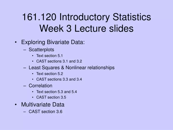
161.120 Introductory Statistics Week 3 Lecture slides

1. 161.120 Introductory Statistics Week 3 Lecture slides • Exploring Bivariate Data: • Scatterplots • Text section 5.1 • CAST sections 3.1 and 3.2 • Least Squares & Nonlinear relationships • Text section 5.2 • CAST sections 3.3 and 3.4 • Correlation • Text section 5.3 and 5.4 • CAST section 3.5 • Multivariate Data • CAST section 3.6

2. Univariate Data • Single measurement from each individual • Cannot associate variation in that measurement with other characteristics of the individuals • all variation is unexplained. • Bivariate Data • Two measurements from each individual • May be be able to associate variation in one measurement with changes in the other measurement • can explain some of the variation. • Examples are ... • Blood pressure and weight of males in their 50s • Carbohydrate content and moisture content of corn • Our aim with such data is to find information about the relationship between the variables.

3. Three Tools we will use … • Scatterplot, a two-dimensional graph of data values • Correlation, a statistic that measures the strength and direction of a linear relationship • Regression equation, an equation that describes the average relationship between a response and explanatory variable

4. Scatterplots • The relationship between two variables cannot be determined from examination of the two variables in isolation.

5. 5.1 Looking for Patterns with Scatterplots Questions to Ask about a Scatterplot • What is the average pattern? Does it look like a straight line or is it curved? • What is the direction of the pattern? • How much do individual points vary from the average pattern? • Are there any unusual data points?

6. Positive/Negative Association • Two variables have a positive association when the values of one variable tend to increase as the values of the other variable increase. • Two variables have a negative association when the values of one variable tend to decrease as the values of the other variable increase.

7. Example 5.1 Height and Handspan Data shown are the first 12 observations of a data set that includes the heights (in inches) and fully stretched handspans (in centimeters) of 167 college students.

8. Example 5.1 Height and Handspan Taller people tend to have greater handspan measurements than shorter people do. When two variables tend to increase together, we say that they have a positive association. The handspan and height measurements may have a linear relationship.

9. Example 5.2 Driver Age and MaximumLegibility Distance of Highway Signs • A research firm determined the maximum distance at which each of 30 drivers could read a newly designed sign. • The 30 participants in the study ranged in age from 18 to 82 years old. • We want to examine the relationship between age and the sign legibility distance.

10. Example 5.2 Driver Age and MaximumLegibility Distance of Highway Signs • We see a negative association with a linear pattern. • We will use a straight-line equation to model this relationship.

11. Example 5.3 The Development of Musical Preferences • The 108 participants in the study ranged in age from 16 to 86 years old. • We want to examine the relationship between song-specific age (age in the year the song was popular) and musical preference (positive score => above average, negative score => below average).

12. Example 5.3 The Development of Musical Preferences • Popular music preferences acquired in late adolescence and early adulthood. • The association is nonlinear.

13. Groups and Outliers • Use different plotting symbols or colors to represent different subgroups. • Look for outliers: points that have an usual combination of data values.

14. In both univariate and bivariate data sets, outliers or clusters must be very distinct before we should conclude that they are real, in the absence of further external information confirming that the individuals are distinct. • Particularly in small data sets, outliers, clusters and other patterns may arise by chance, without being associated with any real features in the individuals. • Be careful not to over interpret features in scatterplot unless they are well defined, especially if the sample size is small.

15. 5.2 Describing Linear Patterns with a Regression Line When the best equation for describing the relationship between x and y is a straight line, the equation is called the regression line. Two purposes of the regression line: • to estimate the average value of y at any specified value of x • to predict the value of y for an individual, given that individual’s x value

16. Example 5.1 Height and Handspan (cont) Regression equation: Handspan = -3 + 0.35 Height Estimate the average handspan for people 60 inches tall:Average handspan = -3 + 0.35(60) = 18 cm. Predict the handspan for someone who is 60 inches tall:Predicted handspan = -3 + 0.35(60) = 18 cm.

17. Example 5.1 Height and Handspan (cont) Regression equation: Handspan = -3 + 0.35 Height Slope = 0.35 => Handspan increases by 0.35 cm, on average, for each increase of 1 inch in height. In a statistical relationship, there is variation from the average pattern.

18. The Equation for the Regression Line is spoken as “y-hat,” and it is also referred to either as predicted y or estimated y. b0 is the intercept of the straight line. The intercept is the value of y when x = 0. b1 is the slope of the straight line. The slope tells us how much of an increase (or decrease) there is for the y variable when the x variable increases by one unit. The sign of the slope tells us whether y increases or decreases when x increases.

19. Example 5.2 Driver Age and MaximumLegibility Distance of Highway Signs (cont) Regression equation: Distance = 577 - 3 Age Slope of –3 tells us that, on average, the legibility distance decreases 3 feet when age increases by one year Estimate the average distance for 20-year-old drivers:Average distance = 577 – 3(20) = 517 ft. Predict the legibility distance for a 20-year-old driver:Predicted distance = 577 – 3(20) = 517 ft.

20. Extrapolation • Usually a bad idea to use a regression equation to predict values faroutside the range where the original data fell. • No guarantee that the relationship will continue beyond the range for which we have observed data.

21. Prediction Errors and Residuals • Prediction Error = difference between the observed value of y and the predicted value . • Residual =

22. x = Age y = Distance Residual 18 510 577 – 3(18)=523 510 – 523 = -13 20 590 577 – 3(20)=517 590 – 517 = 73 22 516 577 – 3(22)=511 516 – 511 = 5 Example 5.2 Driver Age and MaximumLegibility Distance of Highway Signs (cont) Regression equation: = 577 – 3x Can compute the residual for all 30 observations. Positive residual => observed value higher than predicted. Negative residual => observed value lower than predicted.

23. Least Squares Line and Formulas • Least Squares Regression Line: minimizes the sum of squared prediction errors. • SSE = Sum of squared prediction errors. • Formulas for Slope and Intercept:

24. Linear model • Only appropriate when the cloud of crosses in a scatterplot of the data is regularly spread around a straight line. • If the crosses are scattered round a curve, the relationship is called nonlinear and other models must be used. • Outliers should be investigated • Detecting problems with the model • Plot residuals against X to look for problems in the model

25. Nonlinear Relationships • If the relationship between Y and X is nonlinear, a linear model will give poor predictions and must be avoided. • Transformation of one or both variables • often possible to linearise the relationship and therefore use least squares to fit a linear model to the transformed variables • For many data sets, a logarithmic transformation works, but a more general power transformation is sometimes needed to linearise the relationship • Adding a quadratic term • An alternative solution to the problem of curvature is to extend the simple linear model with the addition of a quadratic term

26. 5.3 Measuring Strength and Direction with Correlation Correlation rindicates the strength and the direction of a straight-line relationship. • The strength of the relationship is determined by the closeness of the points to a straight line. • The direction is determined by whether one variable generally increases or generally decreases when the other variable increases.

27. Interpretation of r and a Formula • r is always between –1 and +1 • magnitude indicates the strength • r = –1 or +1 indicates a perfect linear relationship • sign indicates the direction • r = 0 indicates a slope of 0 so knowing x does not change the predicted value of y • Formula for correlation:

29. Example 5.1 Height and Handspan (cont) Regression equation: Handspan = -3 + 0.35 Height Correlation r = +0.74 => a somewhat strong positive linear relationship.

30. Example 5.2 Driver Age and MaximumLegibility Distance of Highway Signs (cont) Correlation r = -0.8=> a somewhatstrong negative linear association. Regression equation: Distance = 577 - 3 Age

31. Example 5.6 Left and Right Handspans If you know the span of a person’s right hand, can you accurately predict his/her left handspan? Correlation r = +0.95 => a verystrong positive linear relationship.

32. Example 5.7 Verbal SAT and GPA Grade point averages (GPAs) and verbal SAT scores for a sample of 100 university students. Correlation r = 0.485 => a moderatelystrong positive linear relationship.

33. Example 5.8 Age and Hours of TV Viewing Relationship between age and hours of daily television viewing for 1913 survey respondents. Correlation r = 0.12 => a weakconnection. Note: a few claimed to watch more than 20 hours/day!

34. Example 5.9 Hours of Sleep and Hours of Study Relationship between reported hours of sleep the previous 24 hours and the reported hours of study during the same period for a sample of 116 college students. Correlation r = –0.36=> a not too strongnegative association.

35. Correlation Coefficient r • Only describes the strength of linear relationships • a good description of the strength of a relationship provided the crosses in a scatterplot of the data are not scattered round a curve. • r may seriously underestimate the strength of a nonlinear relationship. • A scatterplot should always be examined to help assess whether there are features in the data that the correlation coefficient cannot describe. • Nonlinear relationships • Transform the variables to linearise the relationship before evaluating r

36. 5.4 Why the Answers May Not Make Sense • Allowing outliers to overly influence the results • Combining groups inappropriately • Using correlation and a straight-line equation to describe curvilinear data

37. Example 5.4 Height and Foot Length (cont) Three outliers were data entry errors. Regression equation uncorrected data: 15.4 + 0.13 height corrected data: -3.2 + 0.42 height Correlation uncorrected data: r = 0.28 corrected data: r = 0.69

38. Example 5.10 Earthquakes in US San Francisco earthquake of 1906. Correlation all data: r = 0.73 w/o SF: r = –0.96

39. Example 5.11 Height and Lead Feet Scatterplot of all data: College student heights and responses to the question “What is the fastest you have ever driven a car?” Scatterplot by gender: Combining two groups led to illegitimate correlation

40. Example 5.12 Don’t Predict without a Plot Population of US (in millions) for each census year between 1790 and 1990. Correlation: r = 0.96Regression Line: population = –2218 + 1.218(Year)Poor Prediction for Year 2005 = –2218 + 1.218(2005), about 224 million, which is less than the 1990 population.

41. Multivariate Data • Problem: How to display relationship between more than two variables? • An array of scatterplots (matrix plot) of all pairs of variables is often informative • especially if the scatterplots are dynamically linked (brushing).