Download
1 / 30
300 likes | 300 Vues
This study aims to evaluate and improve the representation of mixed-phase clouds in global climate models through the use of radar and lidar observations. It explores the challenges in capturing these clouds and investigates scale-independent parameterizations for their accurate representation. The study also examines the radiative feedback of mixed-phase clouds on climate and investigates the impact of various physical processes on the simulation of these clouds.

E N D
Evaluation and improvement of mixed-phase cloud schemes using radar and lidarobservations Robin Hogan, Andrew Barrett Department of Meteorology, University of Reading Richard Forbes ECMWF
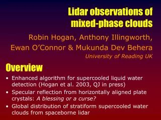
Overview • Why are mixed-phase clouds so poorly captured in GCMs? • These clouds are potentially a key negative feedback for climate • Getting these clouds right requires the correct specification of turbulent mixing, radiation, microphysics, fall speed, sub-grid structure etc. • Vertical resolution is a key issue for representing thin liquid layers • Can we devise a scale-independent parameterization? • Use a 1D model and long-term cloud radar and lidar observations • Easy to perform many sensitivity studies to changed physics
Mixed-phase cloud radiative feedback • Decrease in subtropical stratocumulus • Lower albedo -> positive feedback on climate • Change to cloud mixing ratio on doubling of CO2 • Tsushima et al. (2006) • Increase in polar boundary-layer and mid-latitude mid-level clouds • Clouds more likely to be liquid phase: lower fall speed so more persistent • Higher albedo -> negative climate feedback (Mitchell et al. 1989) • Depends on questionable model physics!
CloudSat & Calipso (Hogan, Stein, Garcon, Delanoe, Forbes, Bodas-Salcedo, in prep.) How well do models capture mid-level clouds? • Ground-based radar and lidar (Illingworth, Hogan et al. 2007) 3.6<t<23 t<3.6 Models miss at least a third of mid-level clouds • ISCCP and CERES (Zhang et al. 2005)
Important processes in altocumulus • Longwave cloud-top cooling • Supercooled droplets form • Cooling induces upside-down convective mixing • Some droplets freeze • Ice particles grow at expense of liquid by Bergeron-Findeisen • Ice particles fall out of layer • Most previous studies (e.g. Xie et al. 2008) in Arctic: surface fluxes important H lE • Many models have prognostic cloud water content, and temperature-dependent ice/liquid split, with less liquid at colder temperatures • Impossible to represent altocumulus clouds properly! • Newer models have separate prognostic ice and liquid mixing ratios • Are they better at mixed-phase clouds?
Observations of long-lived liquid layer • Radar reflectivity (large particles) • Lidar backscatter (small particles) Liquid at –20C • Estimate ice water content from radar reflectivity factor and temperature • Estimate liquid water content from microwave radiometer using scaled adiabatic method
21 altocumulus days at Chilbolton • Met Office models (mesoscale and global) have most sophisticated cloud scheme • Separate prognostic liquid and ice • But these models have the worst supercooled liquid water content and liquid cloud fraction • What are we doing wrong in these schemes?
1D “EMPIRE” model Variables conserved under moist adiabatic processes: Total water (vapour plus liquid): Liquid water potential temperature • Single column model • High vertical resolution • Default: Dz = 50m • Five prognostic variables • u, v, θl, qtand qi • Default: follows Met Office model • Wilson & Ballard microphysics • Local and non-local mixing • Explicit cloud-top entrainment • Frequent radiation updates (Edwards & Slingo scheme) • Advective forcing using ERA-Interim • Flexible: very easy to try different parameterization schemes • Coded in matlab • Each configuration compared to set of 21 Chilbolton altocumulus days
Evaluation of EMPIRE control model More supercooled liquid than Met Office but still seriously underestimated Note that ice & liquid cloud fraction is diagnosed so errors not so fundamental
Effect of turbulent mixing scheme • Quite a small effect!
Effect of vertical resolution • Take EMPIRE and change physical processes within bounds of parameterized uncertainty • Assess change in simulated mixed-phase clouds Significantly less liquid at 500-m resolution Explains poorer performance of Met Office model Thin liquid layers cannot be resolved
Effect of ice growth rate Liquid water distribution improves in response to any change that reduces the ice growth rate in the cloud Change could be: reduced ice number concentration, increased ice fall speed, reduced ice capacitance But which change is physically justifiable?
Summary of sensitivity tests Main model sensitivities appear to be: • Vertical resolution • Can we parameterize the sub-grid vertical distribution to get the same result in the high and low resolution models? • Ice growth rate • Is there something wrong with the size distribution assumed in models that causes too high an ice growth rate when the ice water content is small? • Ice cloud fraction • In most models this is a function of ice mixing ratio and temperature • We have found from Cloudnet observations that the temperature dependence is unnecessary, and that this significantly improves the ice cloud fraction in clouds warmer than –30C (not shown)
Resolution dependence: idealised simulation Liquid Ice
Resolution dependence Best NWP resolution Typical NWP resolution
Effect 1: thin clouds can be missed θl • Consider a 500-m model level at the top of an altocumulus cloud • Consider prognostic variables ql and qt that lead to ql = 0 qt ql T P1 Gridbox-mean liquid can be parameterized P2 • But layer is well mixed which means that even though prognostic variables are constant with height, T decreases significantly in layer • Therefore a liquid cloud may still be present at the top of the layer
Effect 2: Ice growth too high at cloud top • Diffusional growth: qi = ice mixing ratio, ice diameter RHi = relative humidity with respect to ice • qi zero at cloud top: growth too high dqi RHi qi dt P1 Assume linear qiprofile to enable gridbox-mean growth rate to be estimated: significantly lower than before P2 0 0 100%
Parameterization at work Liquid Ice Liquid Ice
Parameterization at work • New parameterization works well over full range of model resolutions • Typically applied only at cloud top, which can be identified objectively
“Marshall-Palmer” inverse exponential used in all situations Simply adjust slope to match ice water content Wilson and Ballard scheme used by Met Office Similar schemes in many other models But how does calculated growth rate versus ice water content compare to calculations from aircraft spectra? Standard ice particle size distribution log(N) N0 = 2x10⁶ Increasing ice water content D
Parameterized growth rates log(N) • Ice clouds with low water content: • Ice growth rate too high • Fall speed too low • Liquid clouds depleted too quickly! Ice growth rate D Ratio of parameterization to aircraft spectra N0 = constant Fall speed Ice water content
Adjusted growth rates log(N) New ice size distribution leads to better agreement in liquid water content • Delanoe and Hogan (2008) suggest N0 smaller for low water content • Much better growth rate and fall speed • Need to account for ice shattering! Ice growth rate D N0 ~ IWC3/4 Ratio of parameterization to aircraft spectra Fall speed Ice water content
Conclusions • Why are mixed-phase clouds so poorly captured in GCMs? • Two key effects that lead to ice growth too fast at cloud top • Sub-grid structure in the vertical • Strong resolution dependence near cloud top; can be parameterized to allow liquid layers that only partially fill the layer vertically • We have parameterized effect on liquid occurrence and ice growth • Error in assumed ice size distribution • More realistic size distribution has fewer, larger crystals at cloud top • Lower ice growth and faster fall speeds so liquid depleted more slowly • Implications for large scale models • NWP: Richard Forbes shown large surface temperature errors unless cloud-top ice growth scaled back: now has physical basis • Climate: urgent need to re-evaluate mixed-phase cloud contribution to climate sensitivity using models with better physics
Radiative properties • Using Edwards and Slingo (1996) radiation code • Water content in different phase can have different radiative impact
Ice particle size distribution • Large ice crystals are more massive and grow faster than smaller crystals • Small crystals have largest impact on growth rate
Cloudnet processing Illingworth, Hogan et al. (BAMS 2007) • Use radar, lidar and microwave radiometer to estimate ice and liquid water content on model grid
Mixed-phase altocumulus clouds Small supercooled liquid cloud droplets • Low fall speed • Highly reflective to sunlight • Often in layers only 100-200 m thick Large ice particles • High fall speed • Much less reflective for a given water content