Download
1 / 46
460 likes | 553 Vues
Velocity Detection of Plasma Patterns from 2D BES Data. Young-chul Ghim(Kim) 1,2 , Anthony Field 2 , Sandor Zoletnik 3 1 Rudolf Peierls Centre for Theoretical Physics, University of Oxford 2 EURATOM/CCFE Fusion Association, Culham, U.K. 3 KFKI RMKI, Association EURATOM/HAS.

E N D
Velocity Detection of Plasma Patternsfrom2D BES Data Young-chul Ghim(Kim)1,2, Anthony Field2, Sandor Zoletnik3 1 Rudolf Peierls Centre for Theoretical Physics, University of Oxford 2 EURATOM/CCFE Fusion Association, Culham, U.K. 3KFKI RMKI, Association EURATOM/HAS
Contents • Brief description of zonal flows, sZFs, and GAMs • Density fluctuation from DIII-D data using CUDA • Meaning of measured velocity from 2D BES data • Detectable range of velocity • How the study is performed. • Mean flow • Temporally fluctuation flow (i.e. GAMs) • Velocity measurements from DIII-D Data • Conclusion
ZFs are not divergence free in a tokamak. A Flux Surface (q=2 surface) 2π (out-board) B-field Zonal Flow: VZF(θ) π (in-board) θ (poloidal) 0 (out-board) 0 π 2π ϕ (toroidal)
So, consequences are generating sZF and/or GAMs. A Flux Surface (q=2 surface) 2π (out-board) B-field Zonal Flow: VZF(θ) sZF and/or GAMs π (in-board) θ (poloidal) 0 (out-board) 0 π 2π ϕ (toroidal)
Structure of GAMs: (m, n) = (0, 0) and (1, 0) Both modes have the same temporal behavior: Spatial structure of GAMs Winsor et al. Phys. Fluids 11, 2448 (1968)
Density response to GAMs Temporal behavior of density fluctuation: Due to m = 0 mode of GAM: Due to m = 1 mode of GAM:
Detecting ñGAM using 2D BES • BES cannot detect m=1 mode of ñGAM because observation position is mid-plane. • How about m= 0 mode of ñGAM? Krämer-Flecken et al. Phy. Rev. Lett. 97, 045006 (2006)
BES can detect GAMs from motions of ñ. To the perpendicular direction on a given flux surface: These induce oscillating perpendicular motion of ñ. To the radial direction: These induce oscillating radial motion of ñ. But, their magnitudes may be small.
Conclusion I • As physicists, we want to know • how zonal flows are generated. • how they suppress turbulence. First, we need to confirm existence of zonal flows. Try to observe ñ associated with zonal flows. In general, not easy. Try to observe ñ associated with GAMs. Hard with BES at the midplane Try to observe GAM induced motions of ñ Possible with BES
Contents • Brief description of zonal flows, sZFs, and GAMs • Density fluctuation from DIII-D data using CUDA • Meaning of measured velocity from 2D BES data • Detectable range of velocity • How the study is performed. • Mean flow • Temporally fluctuation flow (i.e. GAMs) • Velocity measurements from DIII-D Data • Conclusion
DIII-D BES Data • I have two sets of data which each consists of • 7 poloidally separated channesl • with 11 mm separation • for about little bit more than ~ 2 seconds worth • with 1MHz sampling frequency
Data Set #1: Density spectrogram (Ch.1) Some MHD modes? IAW modes?
Contents • Brief description of zonal flows, sZFs, and GAMs • Density fluctuation from DIII-D data using CUDA • Meaning of measured velocity from 2D BES data • Detectable range of velocity • How the study is performed. • Mean flow • Temporally fluctuation flow (i.e. GAMs) • Velocity measurements from DIII-D Data • Conclusion
Mean flows in a tokamak is mostly toroidal. B-field line vplasma = v|| + v θ (poloidal) v|| v (~vExB) vplasma ϕ (toroidal)
Mean flows in a tokamak is mostly toroidal. B-field line vplasma = v|| + v = vϕ + vθ θ (poloidal) v|| v (~vExB) vplasma vθ vϕ ϕ (toroidal)
Poloidal velocity from barber shop effect is close to ExB drift velocity. B-field line vplasma = v|| + v = vϕ + vθ θ (poloidal) v|| vdetected α v vplasma α vθ vϕ ϕ (toroidal)
In addition, we have GAM induced velocity. B-field line θ (poloidal) vGAM vGAMcos(α) v|| vdetected α v vplasma α vθ vϕ ϕ (toroidal)
Conclusion III • We have to be careful when we say ‘poloidal motion’ of a plasma in a tokamak measured by BES. • Poloidal motion of plasma small (on the order of diamagnetic flow) • Poloidal motion of patterns can be on the order of ExB flow (due to ‘barber pole’ effect)
Contents • Brief description of zonal flows, sZFs, and GAMs • Density fluctuation from DIII-D data using CUDA • Meaning of measured velocity from 2D BES data • Detectable range of velocity • How the study is performed. • Mean flow • Temporally fluctuation flow (i.e. GAMs) • Velocity measurements from DIII-D Data • Conclusion
Eddies generated by using GPU (CUDA programming) Equation to generate ‘eddies’ Z vz(R,t) t R Assumed that eddies have Gaussian shapes in R, z, and t-directions plus wave structure in z-direction.
Synthetic BES data are generated by using PSFs and generated eddies.
Back-of-envelope calculation of detectable range of mean velocity using CCTD method • Sampling Frequency: 2 MHz 0.5 usec • Adjacent channel distance: 2.0 cm • Farthest apart channel distance: 6.0cm • Life time of an eddy: 15 usec (This plays a role in lower limit.i.e. before an eddy dies away, it needs to be seen by the next channel.)
Numerical results of detecting mean velocities. Upper limit Lower limit
Conclusion IV • We saw upper and lower limits of detectable mean flow velocity using BES with CCTD technique. • Upper Limit is set by • Sampling frequency • Distance from a channel to next one • Lower Limit is set by • Life time of a structure • Distance from a channel to next one • We saw that • The worse the NSR, the harder to detect GAMs • the faster the mean flow, the harder to detect GAMs
Contents • Brief description of zonal flows, sZFs, and GAMs • Density fluctuation from DIII-D data using CUDA • Meaning of measured velocity from 2D BES data • Detectable range of velocity • How the study is performed. • Mean flow • Temporally fluctuation flow (i.e. GAMs) • Velocity measurements from DIII-D Data • Conclusion
Data Set #1: Fluct. vz(t) of plasma patterns Density is filtered 50.0 kHz < f < 100.0 kHz before vz(t) is calculated.
Data Set #1: Fluct. vz(t) of plasma patterns Density is filtered 0.0 kHz < f < 30.0 kHz before vz(t) is calculated.
Conclusion V • As we just saw, detecting GAM features are not straight forward. • It may be helpful to consider radial motions as well since we have radial motions of eddies due to • Polarization drift • Finite poloidal wave-number associated with m=1 mode of GAM • However, we do not know whether these radial motions are big enough to be seen by the 2D BES.
Final Conclusions • Discussed about ZFs, sZFs, and GAMS. • Because of the observation positions of 2D BES, we use GAMs to “confirm” the existence of zonal flows. • Discussed the meaning of poloidal velocities seen by the 2D BES. • BES sees poloidal motions of ‘plasma patterns’ rather than bulk plasmas. • Discussed detectable ranges of poloidal motions using the CCTD method. • Mean vz: sampling freq., ch. separation dist., lifetime of eddies. • Fluct. vz: NSR levels, vGAM/vmean. • DIII-D data showed that we have to be careful for detecting GAM-like features.
Velocity Detection of Plasma Patternsfrom2D BES Data Young-chul Ghim(Kim)1,2, Anthony Field2, Sandor Zoletnik3 1 Rudolf Peierls Centre for Theoretical Physics, University of Oxford 2 Culham Centre for Fusion Energy, Culham, U.K. 3KFKI RMKI, Association EURATOM/HAS
Data Set #2: Density spectrogram (Ch.1) Some MHD modes? Probably LH transition IAW modes?
Data Set #2: Fluct. vz(t) of plasma patterns Density is filtered 50.0 kHz < f < 100.0 kHz before vz(t) is calculated.
Data Set #2: Fluct. vz(t) of plasma patterns Density is filtered 0.0 kHz < f < 30.0 kHz before vz(t) is calculated.